Supported by Dr. Osamu Ogasawara and  . . |
|
Last data update: 2014.03.03 |
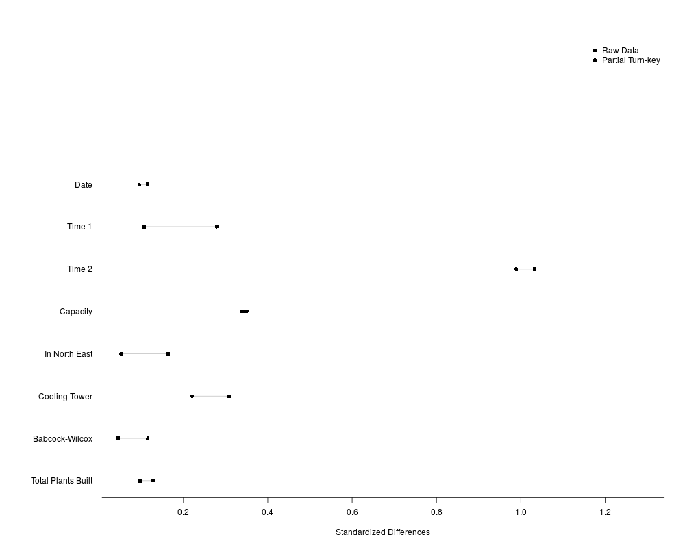
Plot of balance across multiple strataDescriptionThe plot allows a quick visual comparison of the effect of different
stratification designs on the comparability of different
variables. This is not a replacement for the omnibus statistical test
reported as part of Usage## S3 method for class 'xbal' plot(x, xlab = "Standardized Differences", statistic = "std.diff", absolute = FALSE, strata.labels = NULL, variable.labels = NULL, groups = NULL, ...) Arguments
DetailsBy default all variables and all strata are plotted. The scope
of the plot can be reduced by using the
See Also
Examples
data(nuclearplants)
xb <- xBalance(pr ~ date + t1 + t2 + cap + ne + ct + bw + cum.n,
data = nuclearplants,
strata = list("none" = NULL,
"pt" = ~pt))
# Using the default grouping:
plot(xb, variable.labels = c(date = "Date",
t1 = "Time 1",
t2 = "Time 2",
cap = "Capacity",
ne = "In North East",
ct = "Cooling Tower",
bw = "Babcock-Wilcox",
cum.n = "Total Plants Built"),
strata.labels = c("none" = "Raw Data", "pt" = "Partial Turn-key"),
absolute = TRUE)
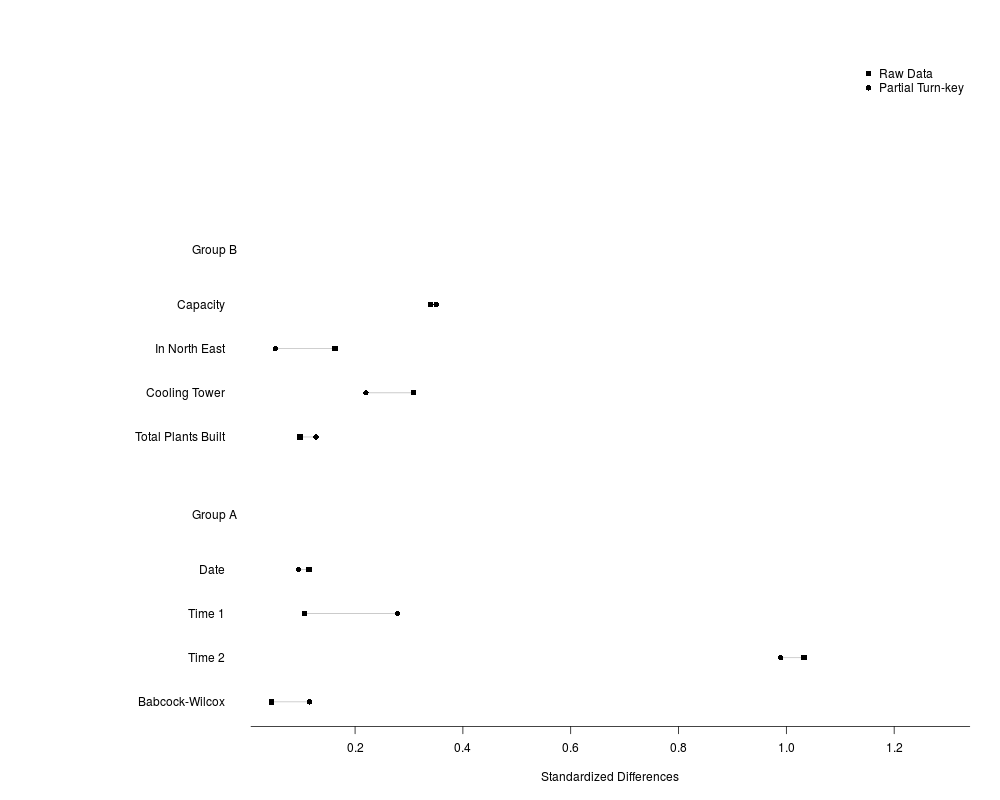
# Using user supplied grouping
plot(xb, variable.labels = c(date = "Date",
t1 = "Time 1",
t2 = "Time 2",
cap = "Capacity",
ne = "In North East",
ct = "Cooling Tower",
bw = "Babcock-Wilcox",
cum.n = "Total Plants Built"),
strata.labels = c("none" = "Raw Data", "pt" = "Partial Turn-key"),
absolute = TRUE,
groups = c("Group A", "Group A", "Group A", "Group B",
"Group B", "Group B", "Group A", "Group B"))
Results
R version 3.3.1 (2016-06-21) -- "Bug in Your Hair"
Copyright (C) 2016 The R Foundation for Statistical Computing
Platform: x86_64-pc-linux-gnu (64-bit)

R is free software and comes with ABSOLUTELY NO WARRANTY.
You are welcome to redistribute it under certain conditions.
Type 'license()' or 'licence()' for distribution details.

R is a collaborative project with many contributors.
Type 'contributors()' for more information and
'citation()' on how to cite R or R packages in publications.

Type 'demo()' for some demos, 'help()' for on-line help, or
'help.start()' for an HTML browser interface to help.
Type 'q()' to quit R.

> library(RItools)
Loading required package: SparseM

Attaching package: 'SparseM'

The following object is masked from 'package:base':

    backsolve

> png(filename="/home/ddbj/snapshot/RGM3/R_CC/result/RItools/plot.xbal.Rd_%03d_medium.png", width=480, height=480)
> ### Name: plot.xbal
> ### Title: Plot of balance across multiple strata
> ### Aliases: plot.xbal
>
> ### ** Examples
>
> data(nuclearplants)
>
> xb <- xBalance(pr ~ date + t1 + t2 + cap + ne + ct + bw + cum.n,
+                data = nuclearplants,
+                strata = list("none" = NULL,
+                    "pt" = ~pt))
>
> # Using the default grouping:
> plot(xb, variable.labels = c(date = "Date",
+              t1 = "Time 1",
+              t2 = "Time 2",
+              cap = "Capacity",
+              ne = "In North East",
+              ct = "Cooling Tower",
+              bw = "Babcock-Wilcox",
+              cum.n = "Total Plants Built"),
+      strata.labels = c("none" = "Raw Data", "pt" = "Partial Turn-key"),
+      absolute = TRUE)
>
> # Using user supplied grouping
> plot(xb, variable.labels = c(date = "Date",
+              t1 = "Time 1",
+              t2 = "Time 2",
+              cap = "Capacity",
+              ne = "In North East",
+              ct = "Cooling Tower",
+              bw = "Babcock-Wilcox",
+              cum.n = "Total Plants Built"),
+      strata.labels = c("none" = "Raw Data", "pt" = "Partial Turn-key"),
+      absolute = TRUE,
+      groups = c("Group A", "Group A", "Group A", "Group B",
+                 "Group B", "Group B", "Group A", "Group B"))
>
>
>
>
>
> dev.off()
null device
          1
>
|