Computes a distance between two partitions of the same data

Description

The function takes as input two partitions of a dataset into clusters, and returns a number which is small if the two partitions are close, large otherwise.

Usage

clScore(c1, c2)

Arguments

Value

A number corresponding to the distance between c1 and c2

Examples

if(require('RUVnormalizeData')){
    
    ## Load the data
    data('gender', package='RUVnormalizeData')
    
    Y <- t(exprs(gender))
    X <- as.numeric(phenoData(gender)$gender == 'M')
    X <- X - mean(X)
    X <- cbind(X/(sqrt(sum(X^2))))
    chip <- annotation(gender)
    
    ## Extract regions and labs for plotting purposes
    lregions <- sapply(rownames(Y),FUN=function(s) strsplit(s,'_')[[1]][2])
    llabs <- sapply(rownames(Y),FUN=function(s) strsplit(s,'_')[[1]][3])
    
    ## Dimension of the factors
    m <- nrow(Y)
    n <- ncol(Y)
    p <- ncol(X)
    
    Y <- scale(Y, scale=FALSE) # Center gene expressions
    
    cIdx <- which(featureData(gender)$isNegativeControl) # Negative control genes
    
    ## Prepare plots
    annot <- cbind(as.character(sign(X)))
    colnames(annot) <- 'gender'
    plAnnots <- list('gender'='categorical')
    lab.and.region <- apply(rbind(lregions, llabs),2,FUN=function(v) paste(v,collapse='_'))
    gender.col <- c('-1' = "deeppink3", '1' = "blue")
    
    ## Remove platform effect by centering.
    
    Y[chip=='hgu95a.db',] <- scale(Y[chip=='hgu95a.db',], scale=FALSE)
    Y[chip=='hgu95av2.db',] <- scale(Y[chip=='hgu95av2.db',], scale=FALSE)
    
    ## Number of genes kept for clustering, based on their variance
    nKeep <- 1260
    
    ##--------------------------
    ## Naive RUV-2 no shrinkage
    ##--------------------------
    
    k <- 20
    nu <- 0
    
    ## Correction
    nsY <- naiveRandRUV(Y, cIdx, nu.coeff=0, k=k)
    
    ## Clustering of the corrected data
    sdY <- apply(nsY, 2, sd)
    ssd <- sort(sdY,decreasing=TRUE,index.return=TRUE)$ix
    kmres2ns <- kmeans(nsY[,ssd[1:nKeep],drop=FALSE],centers=2,nstart=200)
    vclust2ns <- kmres2ns$cluster
    nsScore <- clScore(vclust2ns, X)
    
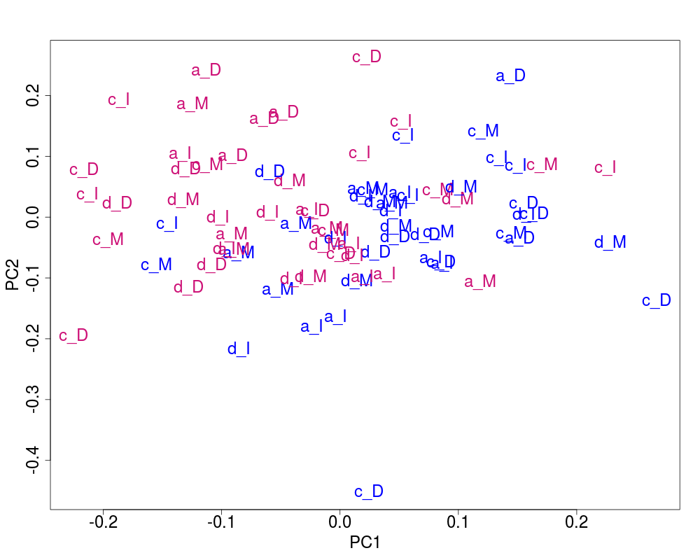
    ## Plot of the corrected data
    svdRes2ns <- NULL
    svdRes2ns <- svdPlot(nsY[, ssd[1:nKeep], drop=FALSE],
                         annot=annot,
                         labels=lab.and.region,
                         svdRes=svdRes2ns,
                         plAnnots=plAnnots,                    
                         kColors=gender.col, file=NULL)   
    
    ##--------------------------
    ## Naive RUV-2 + shrinkage
    ##--------------------------
    
    k <- m
    nu.coeff <- 1e-2
    
    ## Correction
    nY <- naiveRandRUV(Y, cIdx, nu.coeff=nu.coeff, k=k)
    
    ## Clustering of the corrected data
    sdY <- apply(nY, 2, sd)
    ssd <- sort(sdY,decreasing=TRUE,index.return=TRUE)$ix
    kmres2 <- kmeans(nY[,ssd[1:nKeep],drop=FALSE],centers=2,nstart=200)
    vclust2 <- kmres2$cluster
    nScore <- clScore(vclust2,X)
    
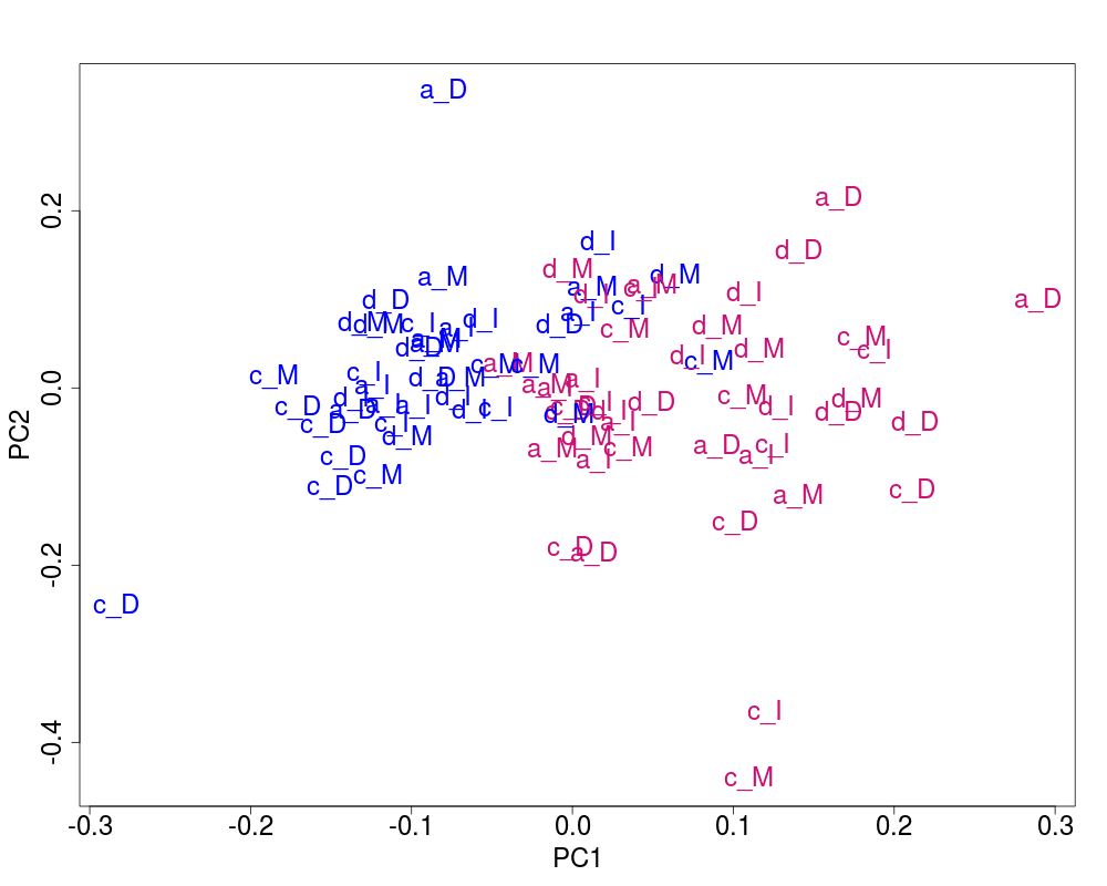
    ## Plot of the corrected data
    svdRes2 <- NULL
    svdRes2 <- svdPlot(nY[, ssd[1:nKeep], drop=FALSE],
                       annot=annot,
                       labels=lab.and.region,
                       svdRes=svdRes2,
                       plAnnots=plAnnots,                    
                       kColors=gender.col, file=NULL)   
}

Results

R version 3.3.1 (2016-06-21) -- "Bug in Your Hair"
Copyright (C) 2016 The R Foundation for Statistical Computing
Platform: x86_64-pc-linux-gnu (64-bit)

R is free software and comes with ABSOLUTELY NO WARRANTY.
You are welcome to redistribute it under certain conditions.
Type 'license()' or 'licence()' for distribution details.

R is a collaborative project with many contributors.
Type 'contributors()' for more information and
'citation()' on how to cite R or R packages in publications.

Type 'demo()' for some demos, 'help()' for on-line help, or
'help.start()' for an HTML browser interface to help.
Type 'q()' to quit R.

> library(RUVnormalize)
> png(filename="/home/ddbj/snapshot/RGM3/R_BC/result/RUVnormalize/clScore.Rd_%03d_medium.png", width=480, height=480)
> ### Name: clScore
> ### Title: Computes a distance between two partitions of the same data
> ### Aliases: clScore
> 
> ### ** Examples
> 
> if(require('RUVnormalizeData')){
+     
+     ## Load the data
+     data('gender', package='RUVnormalizeData')
+     
+     Y <- t(exprs(gender))
+     X <- as.numeric(phenoData(gender)$gender == 'M')
+     X <- X - mean(X)
+     X <- cbind(X/(sqrt(sum(X^2))))
+     chip <- annotation(gender)
+     
+     ## Extract regions and labs for plotting purposes
+     lregions <- sapply(rownames(Y),FUN=function(s) strsplit(s,'_')[[1]][2])
+     llabs <- sapply(rownames(Y),FUN=function(s) strsplit(s,'_')[[1]][3])
+     
+     ## Dimension of the factors
+     m <- nrow(Y)
+     n <- ncol(Y)
+     p <- ncol(X)
+     
+     Y <- scale(Y, scale=FALSE) # Center gene expressions
+     
+     cIdx <- which(featureData(gender)$isNegativeControl) # Negative control genes
+     
+     ## Prepare plots
+     annot <- cbind(as.character(sign(X)))
+     colnames(annot) <- 'gender'
+     plAnnots <- list('gender'='categorical')
+     lab.and.region <- apply(rbind(lregions, llabs),2,FUN=function(v) paste(v,collapse='_'))
+     gender.col <- c('-1' = "deeppink3", '1' = "blue")
+     
+     ## Remove platform effect by centering.
+     
+     Y[chip=='hgu95a.db',] <- scale(Y[chip=='hgu95a.db',], scale=FALSE)
+     Y[chip=='hgu95av2.db',] <- scale(Y[chip=='hgu95av2.db',], scale=FALSE)
+     
+     ## Number of genes kept for clustering, based on their variance
+     nKeep <- 1260
+     
+     ##--------------------------
+     ## Naive RUV-2 no shrinkage
+     ##--------------------------
+     
+     k <- 20
+     nu <- 0
+     
+     ## Correction
+     nsY <- naiveRandRUV(Y, cIdx, nu.coeff=0, k=k)
+     
+     ## Clustering of the corrected data
+     sdY <- apply(nsY, 2, sd)
+     ssd <- sort(sdY,decreasing=TRUE,index.return=TRUE)$ix
+     kmres2ns <- kmeans(nsY[,ssd[1:nKeep],drop=FALSE],centers=2,nstart=200)
+     vclust2ns <- kmres2ns$cluster
+     nsScore <- clScore(vclust2ns, X)
+     
+     ## Plot of the corrected data
+     svdRes2ns <- NULL
+     svdRes2ns <- svdPlot(nsY[, ssd[1:nKeep], drop=FALSE],
+                          annot=annot,
+                          labels=lab.and.region,
+                          svdRes=svdRes2ns,
+                          plAnnots=plAnnots,                    
+                          kColors=gender.col, file=NULL)   
+     
+     ##--------------------------
+     ## Naive RUV-2 + shrinkage
+     ##--------------------------
+     
+     k <- m
+     nu.coeff <- 1e-2
+     
+     ## Correction
+     nY <- naiveRandRUV(Y, cIdx, nu.coeff=nu.coeff, k=k)
+     
+     ## Clustering of the corrected data
+     sdY <- apply(nY, 2, sd)
+     ssd <- sort(sdY,decreasing=TRUE,index.return=TRUE)$ix
+     kmres2 <- kmeans(nY[,ssd[1:nKeep],drop=FALSE],centers=2,nstart=200)
+     vclust2 <- kmres2$cluster
+     nScore <- clScore(vclust2,X)
+     
+     ## Plot of the corrected data
+     svdRes2 <- NULL
+     svdRes2 <- svdPlot(nY[, ssd[1:nKeep], drop=FALSE],
+                        annot=annot,
+                        labels=lab.and.region,
+                        svdRes=svdRes2,
+                        plAnnots=plAnnots,                    
+                        kColors=gender.col, file=NULL)   
+ }
Loading required package: RUVnormalizeData
Loading required package: Biobase
Loading required package: BiocGenerics
Loading required package: parallel

Attaching package: 'BiocGenerics'

The following objects are masked from 'package:parallel':

    clusterApply, clusterApplyLB, clusterCall, clusterEvalQ,
    clusterExport, clusterMap, parApply, parCapply, parLapply,
    parLapplyLB, parRapply, parSapply, parSapplyLB

The following objects are masked from 'package:stats':

    IQR, mad, xtabs

The following objects are masked from 'package:base':

    Filter, Find, Map, Position, Reduce, anyDuplicated, append,
    as.data.frame, cbind, colnames, do.call, duplicated, eval, evalq,
    get, grep, grepl, intersect, is.unsorted, lapply, lengths, mapply,
    match, mget, order, paste, pmax, pmax.int, pmin, pmin.int, rank,
    rbind, rownames, sapply, setdiff, sort, table, tapply, union,
    unique, unsplit

Welcome to Bioconductor

    Vignettes contain introductory material; view with
    'browseVignettes()'. To cite Bioconductor, see
    'citation("Biobase")', and for packages 'citation("pkgname")'.

Warning message:
In naiveRandRUV(Y, cIdx, nu.coeff = nu.coeff, k = k) :
  k larger than the rank of Y[, cIdx]. Using k=82 instead
> 
> 
> 
> 
> 
> dev.off()
null device 
          1 
>