Remove unwanted variation from a gene expression matrix using negative control genes

Description

The function takes as input a gene expression matrix as well as the index of negative control genes. It estimates unwanted variation from these control genes, and removes them by regression, using ridge and/or rank regularization.

Usage

naiveRandRUV(Y, cIdx, nu.coeff=0.001, k=min(nrow(Y), length(cIdx)), tol=1e-6)

Arguments

Details

In terms of model, the rank k can be thought of as the number of independent sources of unwanted variation in the data (i.e., if one source is a linear combination of other sources, it does not increase the rank). The ridge nu.coeff should be inversely proportional to the (expected) magnitude of the unwanted variation.

In practice, even if the real number of independent sources of unwanted variation (resp. their magnitude) is known, using a smaller k (resp., larger ridge) could yield better corrections because one may not have enough samples to effectively estimate all the effects.

More intuition and guidance on the practical choice of these parameters are available in the paper (http://biostatistics.oxfordjournals.org/content/17/1/16.full) and its supplement (http://biostatistics.oxfordjournals.org/content/suppl/2015/08/17/kxv026.DC1/kxv026supp.pdf). In particular: - Equation 2.3 in the manuscript gives an interpretation of the ridge parameter in terms of a probabilistic model. - Section 5.1 of the manuscript provides guidelines to select both parameters on real data. - Section 3 of the supplement compares the effect of reducing the rank and increasing the ridge. - Section 4 of the supplement gives a detailed discussion of how to select the ridge parameter on a real example.

Value

A matrix corresponding to the gene expression after substraction of the estimated unwanted variation term.

Examples

    if(require('RUVnormalizeData')){
     
         ## Load the data
         data('gender', package='RUVnormalizeData')
     
         Y <- t(exprs(gender))
         X <- as.numeric(phenoData(gender)$gender == 'M')
         X <- X - mean(X)
         X <- cbind(X/(sqrt(sum(X^2))))
         chip <- annotation(gender)
             
         ## Extract regions and labs for plotting purposes
         lregions <- sapply(rownames(Y),FUN=function(s) strsplit(s,'_')[[1]][2])
         llabs <- sapply(rownames(Y),FUN=function(s) strsplit(s,'_')[[1]][3])
     
         ## Dimension of the factors
         m <- nrow(Y)
         n <- ncol(Y)
         p <- ncol(X)
     
         Y <- scale(Y, scale=FALSE) # Center gene expressions
     
         cIdx <- which(featureData(gender)$isNegativeControl) # Negative control genes
     
         ## Prepare plots
         annot <- cbind(as.character(sign(X)))
         colnames(annot) <- 'gender'
         plAnnots <- list('gender'='categorical')
         lab.and.region <- apply(rbind(lregions, llabs),2,FUN=function(v) paste(v,collapse='_'))
         gender.col <- c('-1' = "deeppink3", '1' = "blue")
     
         ## Remove platform effect by centering.
     
         Y[chip=='hgu95a.db',] <- scale(Y[chip=='hgu95a.db',], scale=FALSE)
         Y[chip=='hgu95av2.db',] <- scale(Y[chip=='hgu95av2.db',], scale=FALSE)
     
         ## Number of genes kept for clustering, based on their variance
         nKeep <- 1260
     
         ##--------------------------
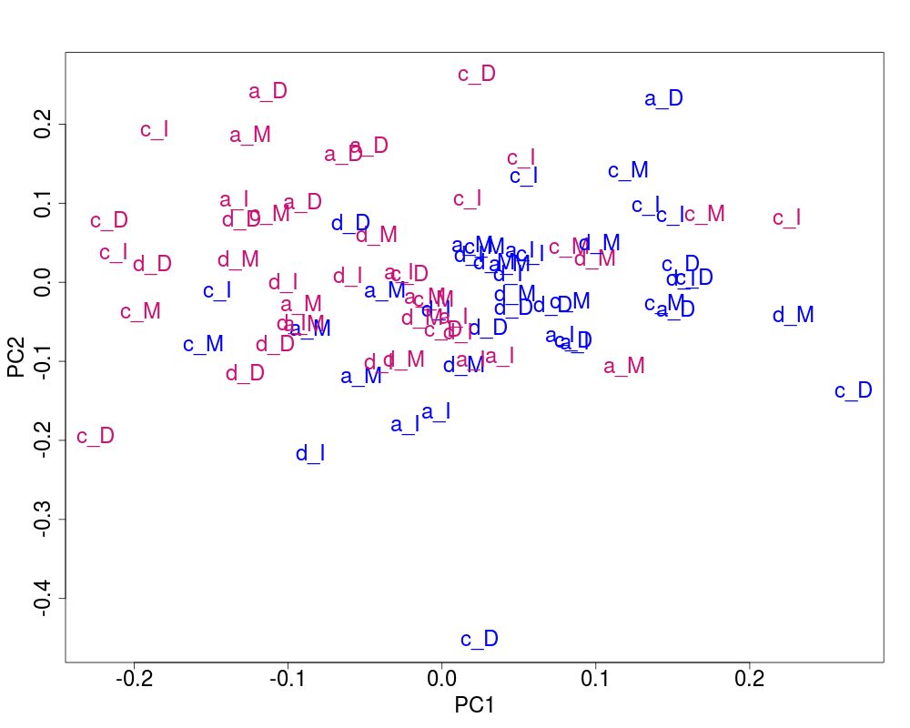
         ## Naive RUV-2 no shrinkage
         ##--------------------------
     
         k <- 20
         nu <- 0
     
         ## Correction
         nsY <- naiveRandRUV(Y, cIdx, nu.coeff=0, k=k)
     
         ## Clustering of the corrected data
         sdY <- apply(nsY, 2, sd)
         ssd <- sort(sdY,decreasing=TRUE,index.return=TRUE)$ix
       kmres2ns <- kmeans(nsY[,ssd[1:nKeep],drop=FALSE],centers=2,nstart=200)
         vclust2ns <- kmres2ns$cluster
         nsScore <- clScore(vclust2ns, X)
     
         ## Plot of the corrected data
         svdRes2ns <- NULL
         svdRes2ns <- svdPlot(nsY[, ssd[1:nKeep], drop=FALSE],
                              annot=annot,
                              labels=lab.and.region,
                              svdRes=svdRes2ns,
                              plAnnots=plAnnots,                    
                              kColors=gender.col, file=NULL)   
     
         ##--------------------------
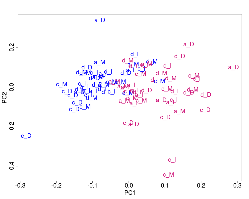
         ## Naive RUV-2 + shrinkage
         ##--------------------------
     
         k <- m
         nu.coeff <- 1e-2
     
         ## Correction
         nY <- naiveRandRUV(Y, cIdx, nu.coeff=nu.coeff, k=k)
     
         ## Clustering of the corrected data
         sdY <- apply(nY, 2, sd)
         ssd <- sort(sdY,decreasing=TRUE,index.return=TRUE)$ix
         kmres2 <- kmeans(nY[,ssd[1:nKeep],drop=FALSE],centers=2,nstart=200)
         vclust2 <- kmres2$cluster
         nScore <- clScore(vclust2,X)
     
         ## Plot of the corrected data
         svdRes2 <- NULL
         svdRes2 <- svdPlot(nY[, ssd[1:nKeep], drop=FALSE],
                            annot=annot,
                            labels=lab.and.region,
                            svdRes=svdRes2,
                            plAnnots=plAnnots,                    
                            kColors=gender.col, file=NULL)   
     }

Results

R version 3.3.1 (2016-06-21) -- "Bug in Your Hair"
Copyright (C) 2016 The R Foundation for Statistical Computing
Platform: x86_64-pc-linux-gnu (64-bit)

R is free software and comes with ABSOLUTELY NO WARRANTY.
You are welcome to redistribute it under certain conditions.
Type 'license()' or 'licence()' for distribution details.

R is a collaborative project with many contributors.
Type 'contributors()' for more information and
'citation()' on how to cite R or R packages in publications.

Type 'demo()' for some demos, 'help()' for on-line help, or
'help.start()' for an HTML browser interface to help.
Type 'q()' to quit R.

> library(RUVnormalize)
> png(filename="/home/ddbj/snapshot/RGM3/R_BC/result/RUVnormalize/naiveRandRUV.Rd_%03d_medium.png", width=480, height=480)
> ### Name: naiveRandRUV
> ### Title: Remove unwanted variation from a gene expression matrix using
> ###   negative control genes
> ### Aliases: naiveRandRUV
> 
> ### ** Examples
> 
>     if(require('RUVnormalizeData')){
+      
+          ## Load the data
+          data('gender', package='RUVnormalizeData')
+      
+          Y <- t(exprs(gender))
+          X <- as.numeric(phenoData(gender)$gender == 'M')
+          X <- X - mean(X)
+          X <- cbind(X/(sqrt(sum(X^2))))
+          chip <- annotation(gender)
+              
+          ## Extract regions and labs for plotting purposes
+          lregions <- sapply(rownames(Y),FUN=function(s) strsplit(s,'_')[[1]][2])
+          llabs <- sapply(rownames(Y),FUN=function(s) strsplit(s,'_')[[1]][3])
+      
+          ## Dimension of the factors
+          m <- nrow(Y)
+          n <- ncol(Y)
+          p <- ncol(X)
+      
+          Y <- scale(Y, scale=FALSE) # Center gene expressions
+      
+          cIdx <- which(featureData(gender)$isNegativeControl) # Negative control genes
+      
+          ## Prepare plots
+          annot <- cbind(as.character(sign(X)))
+          colnames(annot) <- 'gender'
+          plAnnots <- list('gender'='categorical')
+          lab.and.region <- apply(rbind(lregions, llabs),2,FUN=function(v) paste(v,collapse='_'))
+          gender.col <- c('-1' = "deeppink3", '1' = "blue")
+      
+          ## Remove platform effect by centering.
+      
+          Y[chip=='hgu95a.db',] <- scale(Y[chip=='hgu95a.db',], scale=FALSE)
+          Y[chip=='hgu95av2.db',] <- scale(Y[chip=='hgu95av2.db',], scale=FALSE)
+      
+          ## Number of genes kept for clustering, based on their variance
+          nKeep <- 1260
+      
+          ##--------------------------
+          ## Naive RUV-2 no shrinkage
+          ##--------------------------
+      
+          k <- 20
+          nu <- 0
+      
+          ## Correction
+          nsY <- naiveRandRUV(Y, cIdx, nu.coeff=0, k=k)
+      
+          ## Clustering of the corrected data
+          sdY <- apply(nsY, 2, sd)
+          ssd <- sort(sdY,decreasing=TRUE,index.return=TRUE)$ix
+        kmres2ns <- kmeans(nsY[,ssd[1:nKeep],drop=FALSE],centers=2,nstart=200)
+          vclust2ns <- kmres2ns$cluster
+          nsScore <- clScore(vclust2ns, X)
+      
+          ## Plot of the corrected data
+          svdRes2ns <- NULL
+          svdRes2ns <- svdPlot(nsY[, ssd[1:nKeep], drop=FALSE],
+                               annot=annot,
+                               labels=lab.and.region,
+                               svdRes=svdRes2ns,
+                               plAnnots=plAnnots,                    
+                               kColors=gender.col, file=NULL)   
+      
+          ##--------------------------
+          ## Naive RUV-2 + shrinkage
+          ##--------------------------
+      
+          k <- m
+          nu.coeff <- 1e-2
+      
+          ## Correction
+          nY <- naiveRandRUV(Y, cIdx, nu.coeff=nu.coeff, k=k)
+      
+          ## Clustering of the corrected data
+          sdY <- apply(nY, 2, sd)
+          ssd <- sort(sdY,decreasing=TRUE,index.return=TRUE)$ix
+          kmres2 <- kmeans(nY[,ssd[1:nKeep],drop=FALSE],centers=2,nstart=200)
+          vclust2 <- kmres2$cluster
+          nScore <- clScore(vclust2,X)
+      
+          ## Plot of the corrected data
+          svdRes2 <- NULL
+          svdRes2 <- svdPlot(nY[, ssd[1:nKeep], drop=FALSE],
+                             annot=annot,
+                             labels=lab.and.region,
+                             svdRes=svdRes2,
+                             plAnnots=plAnnots,                    
+                             kColors=gender.col, file=NULL)   
+      }
Loading required package: RUVnormalizeData
Loading required package: Biobase
Loading required package: BiocGenerics
Loading required package: parallel

Attaching package: 'BiocGenerics'

The following objects are masked from 'package:parallel':

    clusterApply, clusterApplyLB, clusterCall, clusterEvalQ,
    clusterExport, clusterMap, parApply, parCapply, parLapply,
    parLapplyLB, parRapply, parSapply, parSapplyLB

The following objects are masked from 'package:stats':

    IQR, mad, xtabs

The following objects are masked from 'package:base':

    Filter, Find, Map, Position, Reduce, anyDuplicated, append,
    as.data.frame, cbind, colnames, do.call, duplicated, eval, evalq,
    get, grep, grepl, intersect, is.unsorted, lapply, lengths, mapply,
    match, mget, order, paste, pmax, pmax.int, pmin, pmin.int, rank,
    rbind, rownames, sapply, setdiff, sort, table, tapply, union,
    unique, unsplit

Welcome to Bioconductor

    Vignettes contain introductory material; view with
    'browseVignettes()'. To cite Bioconductor, see
    'citation("Biobase")', and for packages 'citation("pkgname")'.

Warning message:
In naiveRandRUV(Y, cIdx, nu.coeff = nu.coeff, k = k) :
  k larger than the rank of Y[, cIdx]. Using k=82 instead
> 
> 
> 
> 
> 
> dev.off()
null device 
          1 
>