R Graphical Manual

Browse All

Last data update: 2014.03.03

R: Maximum Likelihood Estimation of Effects in Least Angle...

RXlarlso

R Documentation

Maximum Likelihood Estimation of Effects in Least Angle Regression

Description

Identify whether least angle regression estimates are generalized ridge shrinkage estimates and generate TRACE displays for estimates that do correspond to ridge shrinkage factors between 0.00 and 0.99.

Usage

RXlarlso(form, data, rscale = 1, type = "lar", trace = FALSE, 
         eps = .Machine$double.eps, omdmin = 9.9e-13, ...)

Arguments

`form`	A regression formula [y~x1+x2+...] suitable for use with lm().
`data`	Data frame containing observations on all variables in the formula.
`rscale`	One of three possible choices (0, 1 or 2) for rescaling of variables as they are being "centered" to remove non-essential ill-conditioning: 0 implies no rescaling; 1 implies divide each variable by its standard error; 2 implies rescale as in option 1 but re-express answers as in option 0.
`type`	One of "lasso", "lar" or "forward.stagewise" for function lars(). Names can be abbreviated to any unique substring. Default in RXlarlso() is "lar".
`trace`	If TRUE, lars() function prints out its progress.
`eps`	The effective zero for lars().
`omdmin`	Strictly positive minimum allowed value for one-minus-delta (default = 9.9e-013.)
`...`	Optional argument(s) passed on to the lars() function from the lars R-package.

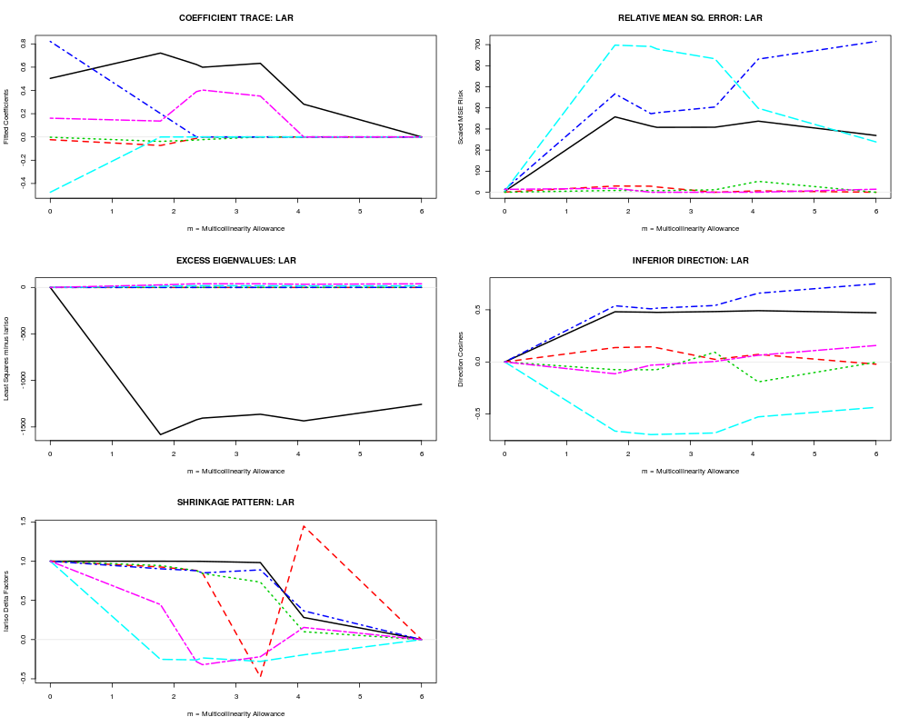
Details

RXlarlso() calls the Efron/Hastie lars() function to perform Least Angle Regression on X-variables that have been centered and possibly rescaled but which may be (highly) correlated. Maximum likelihood TRACE displays paralleling those of RXridge are also computed and (optionally) plotted.

Value

An output list object of class RXlarlso:

`form`	The regression formula specified as the first argument.
`data`	Name of the data.frame object specified as the second argument.
`p`	Number of regression predictor variables.
`n`	Number of complete observations after removal of all missing values.
`r2`	Numerical value of R-square goodness-of-fit statistic.
`s2`	Numerical value of the residual mean square estimate of error.
`prinstat`	Listing of principal statistics.
`gmat`	Orthogonal matrix of direction cosines for regressor principal axes.
`lars`	An object of class lars.
`coef`	Matrix of shrinkage-ridge regression coefficient estimates.
`risk`	Matrix of MSE risk estimates for fitted coefficients.
`exev`	Matrix of excess MSE eigenvalues (ordinary least squares minus ridge.)
`infd`	Matrix of direction cosines for the estimated inferior direction, if any.
`spat`	Matrix of shrinkage pattern multiplicative delta factors.
`mlik`	Listing of criteria for maximum likelihood selection of M-extent-of-shrinkage.
`sext`	Listing of summary statistics for all M-extents-of-shrinkage.

Author(s)

Bob Obenchain <wizbob@att.net>

References

Breiman L. (1995) Better subset regression using the non-negative garrote. Technometrics 37, 373-384.

Efron B, Hastie T, Johnstone I, Tibshirani R. (2004) Least angle regression. Ann. Statis. 32, 407-499.

Obenchain RL. (2005) Shrinkage Regression: ridge, BLUP, Bayes, spline and Stein. Electronic book-in-progress (200+ pages.) http://members.iquest.net/~softrx/

Obenchain RL. (2011) shrink.PDF Vignette-like documentation stored in the R library/RXshrink/doc folder. 23 pages.

Tibshirani R. (1996) Regression shrinkage and selection via the lasso. J. Roy. Stat. Soc. B 58, 267-288.

Examples

  data(longley2)
  form <- GNP~GNP.deflator+Unemployed+Armed.Forces+Population+Year+Employed
  rxlobj <- RXlarlso(form, data=longley2)
  rxlobj
  names(rxlobj)
  plot(rxlobj)

Results


R version 3.3.1 (2016-06-21) -- "Bug in Your Hair"
Copyright (C) 2016 The R Foundation for Statistical Computing
Platform: x86_64-pc-linux-gnu (64-bit)

R is free software and comes with ABSOLUTELY NO WARRANTY.
You are welcome to redistribute it under certain conditions.
Type 'license()' or 'licence()' for distribution details.

R is a collaborative project with many contributors.
Type 'contributors()' for more information and
'citation()' on how to cite R or R packages in publications.

Type 'demo()' for some demos, 'help()' for on-line help, or
'help.start()' for an HTML browser interface to help.
Type 'q()' to quit R.

> library(RXshrink)
Loading required package: lars
Loaded lars 1.2

> png(filename="/home/ddbj/snapshot/RGM3/R_CC/result/RXshrink/RXlarlso.Rd_%03d_medium.png", width=480, height=480)
> ### Name: RXlarlso
> ### Title: Maximum Likelihood Estimation of Effects in Least Angle
> ###   Regression
> ### Aliases: RXlarlso
> ### Keywords: regression hplot
> 
> ### ** Examples
> 
>   data(longley2)
>   form <- GNP~GNP.deflator+Unemployed+Armed.Forces+Population+Year+Employed
>   rxlobj <- RXlarlso(form, data=longley2)
>   rxlobj

RXlarlso Object: LARS Maximum Likelihood Shrinkage
Data Frame: longley2 
Regression Equation:
GNP ~ GNP.deflator + Unemployed + Armed.Forces + Population + 
    Year + Employed

    Number of Regressor Variables, p = 6 
    Number of Observations, n = 29 

Principal Axis Summary Statistics of Ill-Conditioning...
        LAMBDA         SV         COMP         RHO       TRAT
1 124.55432117 11.1603907  0.466590166  0.98409260 179.451944
2  34.04395492  5.8347198 -0.009779055 -0.01078296  -1.966301
3   7.97601572  2.8241841  0.228918857  0.12217872  22.279619
4   1.31429584  1.1464274 -0.557948473 -0.12088200 -22.043160
5   0.06505309  0.2550551  0.613987118  0.02959472   5.396677
6   0.04635925  0.2153120 -0.471410409 -0.01918176  -3.497845

    Residual Mean Square for Error = 0.0008420418 
    Estimate of Residual Std. Error = 0.02901796 


The extent of shrinkage (M value) most likely to be optimal
depends upon whether one uses the Classical, Empirical Bayes, or
Random Coefficient criterion.  In each case, the objective is to
minimize the minus-two-log-likelihood statistics listed below:
         M         CLIK       EBAY      RCOF
0 0.000000          Inf        Inf       Inf
1 1.781335 8.028865e+01   143.8218  71.61305
2 2.362316 1.031755e+02   232.0318  82.12630
3 2.460471 1.086027e+02   280.2866  86.52931
4 3.395439 1.557455e+02   810.7413 112.66440
5 4.096776 1.009984e+12 23947.7492 231.47905
6 6.000000 2.123044e+02 33230.5079 212.30445

Extent of shrinkage statistics...
       TSMSE     MCAL
0   37.86637 0.000000
1 1578.48713 1.781335
2 1413.97919 2.362316
3 1396.36404 2.460471
4 1357.07572 3.395439
5 1425.20255 4.096776
6 1237.17669 6.000000

Output from LARS invocation...

Call:
lars(x = crx, y = cry, type = type, trace = trace, normalize = eps)
R-squared: 0.999 
Sequence of LAR moves:
                
Var  1 6 3 2 4 5
Step 1 2 3 4 5 6
>   names(rxlobj)
 [1] "data"     "form"     "p"        "n"        "r2"       "s2"      
 [7] "prinstat" "gmat"     "lars"     "coef"     "rmse"     "exev"    
[13] "infd"     "spat"     "mlik"     "sext"    
>   plot(rxlobj)
> 
> 
> 
> 
> 
> dev.off()
null device 
          1 
>