Maximum Likelihood Shrinkage via Generalized Ridge or Least Angle Regression

Description

The functions in this package augment the basic calculations of Generalized Ridge and Least Angle Regression with important visualization tools. Specifically, they display TRACEs of normal-distribution-theory Maximum Likelihood estimates of the key quantities that completely characterize the effects of shrinkage on the MSE Risk of fitted coefficients.

Details

RXridge() calculates and displays TRACEs for the Q-shaped shrinkage path, including the M-extent of shrinkage along that path, that are most likely under normal distribution theory to yield optimal reducions in MSE Risk.

When regression parameters have specified, KNOWN numerical values, RXtrisk() calculates and displays the corresponding True MSE Risk profiles and RXtsimu() first simulates Y-outcome data then calculates true Squared Error Losss associated with Q-shape shrinkage.

RXlarlso() calls the Efron/Hastie lars() R-function to perform Least Angle Regression then augments these calculations with Maximum Likelihood TRACE displays like those of RXridge().

RXuclars() applies Least Angle Regression to the uncorrelated components of a possibly ill-conditioned set of X-variables using a closed-form expression for the lars/lasso shrinkage delta factors that exits in this special case.

Author(s)

Bob Obenchain <wizbob@att.net>

References

Efron B, Hastie T, Johnstone I, Tibshirani R. (2004) Least angle regression. Ann. Statis. 32, 407-499.

Goldstein M, Smith AFM. (1974) Ridge-type estimators for regression analysis. J. Roy. Stat. Soc. B 36, 284-291. (2-parameter shrinkage family.)

Obenchain RL. (2005) Shrinkage Regression: ridge, BLUP, Bayes, spline and Stein. Electronic book-in-progress (200+ pages.) http://members.iquest.net/~softrx/.

Obenchain RL. (2011) shrink.PDF Vignette-like documentation stored in the R library/RXshrink/doc folder. 23 pages.

Examples

  demo(longley2)

Results

R version 3.3.1 (2016-06-21) -- "Bug in Your Hair"
Copyright (C) 2016 The R Foundation for Statistical Computing
Platform: x86_64-pc-linux-gnu (64-bit)

R is free software and comes with ABSOLUTELY NO WARRANTY.
You are welcome to redistribute it under certain conditions.
Type 'license()' or 'licence()' for distribution details.

R is a collaborative project with many contributors.
Type 'contributors()' for more information and
'citation()' on how to cite R or R packages in publications.

Type 'demo()' for some demos, 'help()' for on-line help, or
'help.start()' for an HTML browser interface to help.
Type 'q()' to quit R.

> library(RXshrink)
Loading required package: lars
Loaded lars 1.2

> png(filename="/home/ddbj/snapshot/RGM3/R_CC/result/RXshrink/RXshrink-package.Rd_%03d_medium.png", width=480, height=480)
> ### Name: RXshrink-package
> ### Title: Maximum Likelihood Shrinkage via Generalized Ridge or Least
> ###   Angle Regression
> ### Aliases: RXshrink-package
> ### Keywords: package
> 
> ### ** Examples
> 
>   demo(longley2)


	demo(longley2)
	---- ~~~~~~~~

>   require(RXshrink)

>   # input revised Longley dataset of Hoerl(2000).
>   data(longley2)

>   # Specify form of regression model (linear here)...
>   form <- GNP~GNP.deflator+Unemployed+Armed.Forces+Population+Year+Employed

>   # Fit of this model using 2-parameter Generalized Ridge Regression
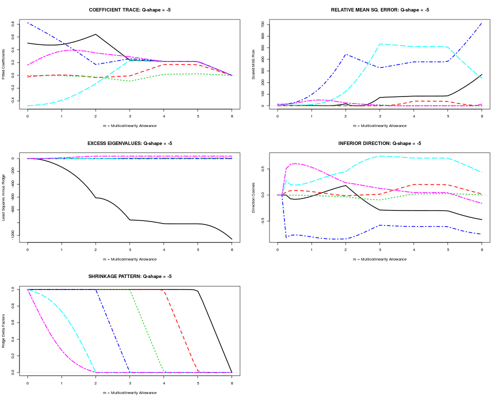
>   rxrobj <- RXridge(form, data=longley2)

>   rxrobj

RXridge Object: Shrinkage-Ridge Regression Model Specification
Data Frame: longley2 
Regression Equation:
GNP ~ GNP.deflator + Unemployed + Armed.Forces + Population + 
    Year + Employed

    Number of Regressor Variables, p = 6 
    Number of Observations, n = 29 

Principal Axis Summary Statistics of Ill-Conditioning...
        LAMBDA         SV         COMP         RHO       TRAT
1 124.55432117 11.1603907  0.466590166  0.98409260 179.451944
2  34.04395492  5.8347198 -0.009779055 -0.01078296  -1.966301
3   7.97601572  2.8241841  0.228918857  0.12217872  22.279619
4   1.31429584  1.1464274 -0.557948473 -0.12088200 -22.043160
5   0.06505309  0.2550551  0.613987118  0.02959472   5.396677
6   0.04635925  0.2153120 -0.471410409 -0.01918176  -3.497845

    Residual Mean Square for Error = 0.0008420418 
    Estimate of Residual Std. Error = 0.02901796 

Classical Maximum Likelihood choice of SHAPE(Q) and EXTENT(M) of
shrinkage in the 2-parameter generalized ridge family...
      Q       CRLQ        M            K    CHISQ
1   5.0 0.03065132 5.973237 9.992836e+06 212.2772
2   4.5 0.03143266 5.971855 2.123279e+06 212.2758
3   4.0 0.03244203 5.970023 4.476833e+05 212.2739
4   3.5 0.03402277 5.967055 9.194427e+04 212.2709
5   3.0 0.03715373 5.960805 1.752828e+04 212.2644
6   2.5 0.04516043 5.942561 2.721213e+03 212.2453
7   2.0 0.07215281 5.858787 2.496728e+02 212.1532
8   1.5 0.18443773 5.252697 9.850159e+00 211.3015
9   1.0 0.52547213 2.111210 5.428963e-01 202.9410
10  0.5 0.79341430 1.816359 4.358166e-01 183.5424
11  0.0 0.89070908 2.678418 1.513692e+00 166.6511
12 -0.5 0.93599740 3.140371 7.907552e+00 151.8817
13 -1.0 0.95935445 3.453422 5.035840e+01 139.1481
14 -1.5 0.97160704 3.723747 3.725912e+02 129.0260
15 -2.0 0.97800933 3.935491 3.139861e+03 121.8070
16 -2.5 0.98131461 4.068103 2.941270e+04 117.2079
17 -3.0 0.98299124 4.168863 2.970284e+05 114.5558
18 -3.5 0.98382102 4.283839 3.143926e+06 113.1458
19 -4.0 0.98421686 4.427912 3.417785e+07 112.4479
20 -4.5 0.98439456 4.586356 3.768549e+08 112.1289
21 -5.0 0.98446554 4.729924 4.185069e+09 112.0005

 Q = -5  is the path shape most likely to lead to minimum
MSE risk because this shape maximizes CRLQ and minimizes CHISQ.


RXridge: Shrinkage PATH Shape = -5 

The extent of shrinkage (M value) most likely to be optimal
in the Q-shape = -5  2-parameter ridge family can depend
upon whether one uses the Classical, Empirical Bayes, or Random
Coefficient criterion.  In each case, the objective is to
minimize the minus-two-log-likelihood statistics listed below:
       M            K         CLIK       EBAY     RCOF
0  0.000 0.000000e+00          Inf        Inf      Inf
1  0.125 1.216886e-09 1.756397e+12   113.2484 113.7283
2  0.250 2.723817e-09 1.759946e+12   112.8258 113.6267
3  0.375 4.619196e-09 1.761921e+12   113.3184 114.2927
4  0.500 7.041824e-09 1.763266e+12   114.2322 115.2383
5  0.625 1.018846e-08 1.764282e+12   115.4263 116.3236
6  0.750 1.433883e-08 1.765097e+12   116.8508 117.4949
7  0.875 1.989252e-08 1.765775e+12   118.4883 118.7274
8  1.000 2.742919e-08 1.766353e+12   120.3319 120.0052
9  1.125 3.782128e-08 1.766854e+12   122.3731 121.3120
10 1.250 5.247015e-08 1.767295e+12   124.5961 122.6278
11 1.375 7.384438e-08 1.767690e+12   126.9746 123.9280
12 1.500 1.068417e-07 1.768051e+12   129.4727 125.1831
13 1.625 1.628770e-07 1.768393e+12   132.0423 126.3550
14 1.750 2.762155e-07 1.701520e+12   134.5264 127.2992
15 1.875 6.182665e-07 1.272220e+12   136.0903 127.1936
16 2.000 6.643946e-04 1.015978e+12   125.4323 114.7166
17 2.125 7.362916e-01 3.287066e+10   166.0541 114.1279
18 2.250 1.717996e+00 3.205070e+10   224.4040 123.2937
19 2.375 3.092344e+00 3.183538e+10   283.5606 129.9525
20 2.500 5.153758e+00 2.280920e+10   342.6568 134.7201
21 2.625 8.589062e+00 1.368552e+10   401.6391 138.2106
22 2.750 1.545756e+01 7.604699e+09   460.4319 140.7063
23 2.875 3.603308e+01 3.262206e+09   518.4773 141.8635
24 3.000 1.151864e+03 1.020496e+08   568.7408 134.7453
25 3.125 3.681964e+04 3.192275e+06   620.4632 127.5772
26 3.250 8.582348e+04 1.369417e+06   680.1102 127.9952
27 3.375 1.544348e+05 7.609366e+05   740.5562 128.9705
28 3.500 2.573141e+05 4.566294e+05   801.2635 130.0100
29 3.625 4.286244e+05 2.740626e+05   862.0149 130.9378
30 3.750 7.703843e+05 1.524187e+05   922.6029 131.6017
31 3.875 1.783600e+06 6.576456e+04   982.5073 131.6508
32 4.000 2.001657e+07 5.802433e+03  1034.0751 128.3256
33 4.125 2.246123e+08 5.233168e+02  1037.2882 123.8210
34 4.250 5.199270e+08 2.503376e+02  1039.1120 122.3877
35 4.375 9.341967e+08 1.669789e+02  1042.2842 121.5122
36 4.500 1.555265e+09 1.313719e+02  1047.3773 120.8768
37 4.625 2.588153e+09 1.157462e+02  1056.0587 120.4012
38 4.750 4.641076e+09 1.121409e+02  1073.4679 120.1243
39 4.875 1.062368e+10 1.206503e+02  1124.3692 120.4956
40 5.000 7.624894e+10 1.585962e+02  1675.8231 129.9001
41 5.125 5.472829e+11 1.878722e+02  5146.2928 160.3667
42 5.250 1.252858e+12 1.954643e+02  9119.6085 176.2351
43 5.375 2.246916e+12 1.994637e+02 13126.9105 186.3760
44 5.500 3.740036e+12 2.022119e+02 17143.1003 193.8197
45 5.625 6.229664e+12 2.043992e+02 21162.8987 199.6993
46 5.750 1.120975e+13 2.063548e+02 25184.5175 204.5580
47 5.875 2.615094e+13 2.083713e+02 29207.1835 208.6979
48 6.000          Inf 2.123044e+02 33230.5079 212.3044

Extent of shrinkage statistics...
        TSMSE        KONST  MCAL
0    37.86637 0.000000e+00 0.000
1    35.63211 1.216886e-09 0.125
2    39.12317 2.723817e-09 0.250
3    47.93770 4.619196e-09 0.375
4    61.61001 7.041824e-09 0.500
5    79.63968 1.018846e-08 0.625
6   101.56149 1.433883e-08 0.750
7   127.06069 1.989252e-08 0.875
8   156.63450 2.742919e-08 1.000
9   190.20102 3.782128e-08 1.125
10  228.25031 5.247015e-08 1.250
11  271.54570 7.384438e-08 1.375
12  321.12648 1.068417e-07 1.500
13  379.33422 1.628770e-07 1.625
14  446.84128 2.762155e-07 1.750
15  524.02860 6.182665e-07 1.875
16  611.40396 6.643946e-04 2.000
17  616.62297 7.362916e-01 2.125
18  634.98390 1.717996e+00 2.250
19  662.37733 3.092344e+00 2.375
20  694.87755 5.153758e+00 2.500
21  741.92078 8.589062e+00 2.625
22  799.43676 1.545756e+01 2.750
23  867.39853 3.603308e+01 2.875
24  942.97404 1.151864e+03 3.000
25  946.23548 3.681964e+04 3.125
26  949.33386 8.582348e+04 3.250
27  955.90253 1.544348e+05 3.375
28  964.03468 2.573141e+05 3.500
29  973.73298 4.286244e+05 3.625
30  984.99979 7.703843e+05 3.750
31  997.81842 1.783600e+06 3.875
32 1010.78728 2.001657e+07 4.000
33 1012.16892 2.246123e+08 4.125
34 1012.23283 5.199270e+08 4.250
35 1012.24831 9.341967e+08 4.375
36 1012.25508 1.555265e+09 4.500
37 1012.26255 2.588153e+09 4.625
38 1012.27763 4.641076e+09 4.750
39 1012.32214 1.062368e+10 4.875
40 1012.83817 7.624894e+10 5.000
41 1018.54240 5.472829e+11 5.125
42 1030.33840 1.252858e+12 5.250
43 1047.92954 2.246916e+12 5.375
44 1071.29714 3.740036e+12 5.500
45 1100.43720 6.229664e+12 5.625
46 1135.37352 1.120975e+13 5.750
47 1181.88392 2.615094e+13 5.875
48 1237.17669          Inf 6.000

>   names(rxrobj)
 [1] "data"     "form"     "p"        "n"        "r2"       "s2"      
 [7] "prinstat" "crlqstat" "qmse"     "qp"       "coef"     "rmse"    
[13] "exev"     "infd"     "spat"     "mlik"     "sext"    

>   plot(rxrobj)

>   cat("\n Press ENTER for Least Angle Regression demo...")

 Press ENTER for Least Angle Regression demo...
>   scan()
1: 
Read 0 items
numeric(0)

>   # Fit of the above model with Least Angle Regression
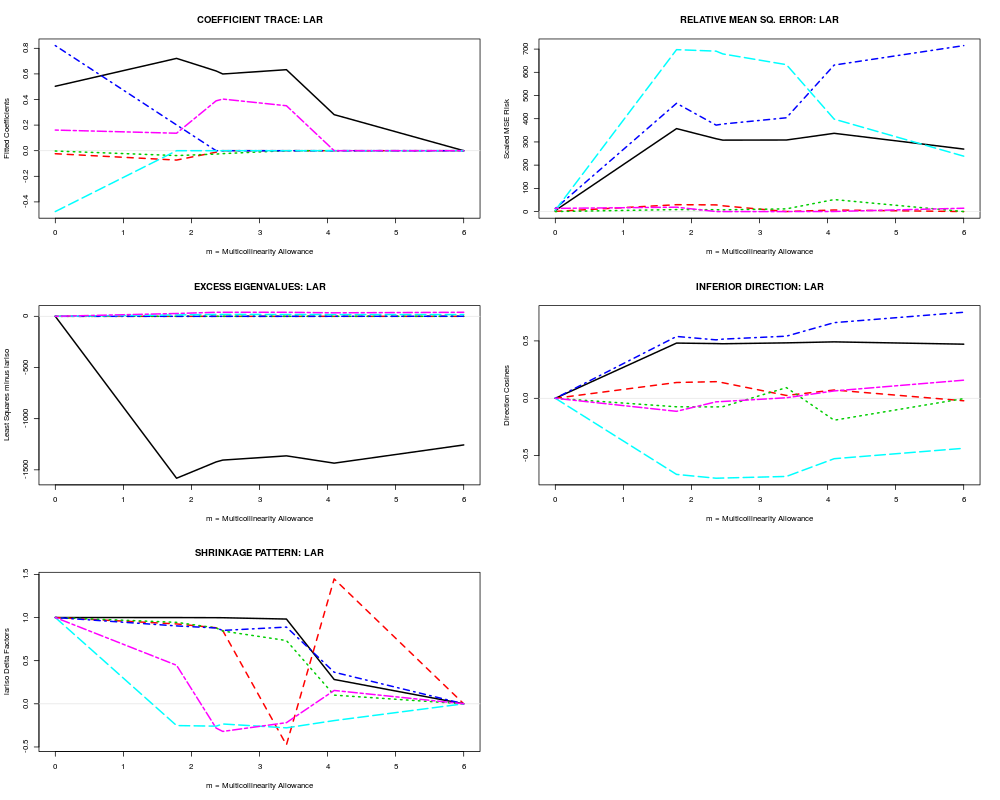
>   rxlobj <- RXlarlso(form, data=longley2)

>   rxlobj

RXlarlso Object: LARS Maximum Likelihood Shrinkage
Data Frame: longley2 
Regression Equation:
GNP ~ GNP.deflator + Unemployed + Armed.Forces + Population + 
    Year + Employed

    Number of Regressor Variables, p = 6 
    Number of Observations, n = 29 

Principal Axis Summary Statistics of Ill-Conditioning...
        LAMBDA         SV         COMP         RHO       TRAT
1 124.55432117 11.1603907  0.466590166  0.98409260 179.451944
2  34.04395492  5.8347198 -0.009779055 -0.01078296  -1.966301
3   7.97601572  2.8241841  0.228918857  0.12217872  22.279619
4   1.31429584  1.1464274 -0.557948473 -0.12088200 -22.043160
5   0.06505309  0.2550551  0.613987118  0.02959472   5.396677
6   0.04635925  0.2153120 -0.471410409 -0.01918176  -3.497845

    Residual Mean Square for Error = 0.0008420418 
    Estimate of Residual Std. Error = 0.02901796 


The extent of shrinkage (M value) most likely to be optimal
depends upon whether one uses the Classical, Empirical Bayes, or
Random Coefficient criterion.  In each case, the objective is to
minimize the minus-two-log-likelihood statistics listed below:
         M         CLIK       EBAY      RCOF
0 0.000000          Inf        Inf       Inf
1 1.781335 8.028865e+01   143.8218  71.61305
2 2.362316 1.031755e+02   232.0318  82.12630
3 2.460471 1.086027e+02   280.2866  86.52931
4 3.395439 1.557455e+02   810.7413 112.66440
5 4.096776 1.009984e+12 23947.7492 231.47905
6 6.000000 2.123044e+02 33230.5079 212.30445

Extent of shrinkage statistics...
       TSMSE     MCAL
0   37.86637 0.000000
1 1578.48713 1.781335
2 1413.97919 2.362316
3 1396.36404 2.460471
4 1357.07572 3.395439
5 1425.20255 4.096776
6 1237.17669 6.000000

Output from LARS invocation...

Call:
lars(x = crx, y = cry, type = type, trace = trace, normalize = eps)
R-squared: 0.999 
Sequence of LAR moves:
                
Var  1 6 3 2 4 5
Step 1 2 3 4 5 6

>   names(rxlobj)
 [1] "data"     "form"     "p"        "n"        "r2"       "s2"      
 [7] "prinstat" "gmat"     "lars"     "coef"     "rmse"     "exev"    
[13] "infd"     "spat"     "mlik"     "sext"    

>   plot(rxlobj)

>   cat("\n Press ENTER for Least Angle fit to Uncorrelated Components...")

 Press ENTER for Least Angle fit to Uncorrelated Components...
>   scan()
1: 
Read 0 items
numeric(0)

>   # Fit Least Angle Regression to Uncorrelated Components (closed form)...
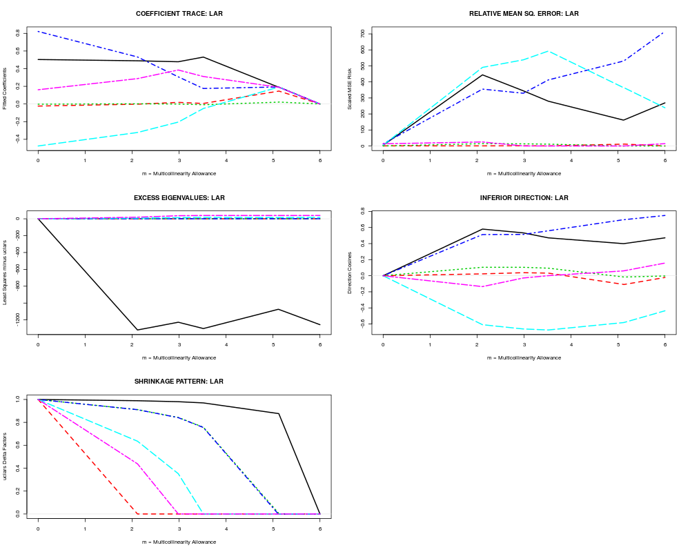
>   rxuobj <- RXuclars(form, data=longley2)

>   rxuobj

RXuclars Object: Uncorrelated Component LARS Shrinkage
Data Frame: longley2 
Regression Equation:
GNP ~ GNP.deflator + Unemployed + Armed.Forces + Population + 
    Year + Employed

    Number of Regressor Variables, p = 6 
    Number of Observations, n = 29 

Principal Axis Summary Statistics of Ill-Conditioning...
        LAMBDA         SV         COMP         RHO       TRAT
1 124.55432117 11.1603907  0.466590166  0.98409260 179.451944
2  34.04395492  5.8347198 -0.009779055 -0.01078296  -1.966301
3   7.97601572  2.8241841  0.228918857  0.12217872  22.279619
4   1.31429584  1.1464274 -0.557948473 -0.12088200 -22.043160
5   0.06505309  0.2550551  0.613987118  0.02959472   5.396677
6   0.04635925  0.2153120 -0.471410409 -0.01918176  -3.497845

    Residual Mean Square for Error = 0.0008420418 
    Estimate of Residual Std. Error = 0.02901796 


The extent of shrinkage (M value) most likely to be optimal
depends upon whether one uses the Classical, Empirical Bayes, or
Random Coefficient criterion.  In each case, the objective is to
minimize the minus-two-log-likelihood statistics listed below:
         M     CLIK       EBAY     RCOF
0 0.000000      Inf        Inf      Inf
1 2.114916 149.4278   472.3079 100.5459
2 2.983319 157.4982   825.7711 113.6821
3 3.517121 164.6308  1259.1945 124.0563
4 5.112223 187.2225  4980.0349 159.4655
5 5.124154 187.5178  5027.7148 159.7195
6 6.000000 212.3044 33230.5079 212.3044

Extent of shrinkage statistics...
       TSMSE     MCAL
0   37.86637 0.000000
1 1330.28575 2.114916
2 1226.23804 2.983319
3 1296.89147 3.517121
4 1068.18888 5.112223
5 1069.64994 5.124154
6 1237.17669 6.000000

Output from LARS invocation...

Call:
lars(x = sx$u, y = cry, type = type, trace = trace, normalize = eps)
R-squared: 0.999 
Sequence of LAR moves:
                
Var  1 3 4 5 6 2
Step 1 2 3 4 5 6

>   plot(rxuobj)
> 
> 
> 
> dev.off()
null device 
          1 
>