R Graphical Manual

Browse All

Last data update: 2014.03.03

R: Maximum Likelihood Least Angle Regression on Uncorrelated...

RXuclars

R Documentation

Maximum Likelihood Least Angle Regression on Uncorrelated X-Components

Description

Apply least angle regression estimation to the uncorrelated components of a possibly ill-conditioned linear regression model and generate normal-theory maximum likelihood TRACE displays.

Usage

  RXuclars(form, data, rscale = 1, type = "lar", trace = FALSE, 
           eps = .Machine$double.eps, omdmin = 9.9e-13, ...)

Arguments

`form`	A regression formula [y~x1+x2+...] suitable for use with lm().
`data`	Data frame containing observations on all variables in the formula.
`rscale`	One of three possible choices (0, 1 or 2) for rescaling of variables as they are being "centered" to remove non-essential ill-conditioning: 0 implies no rescaling; 1 implies divide each variable by its standard error; 2 implies rescale as in option 1 but re-express answers as in option 0.
`type`	One of "lasso", "lar" or "forward.stagewise" for function lars(). Names can be abbreviated to any unique substring. Default in RXlarlso() is "lar".
`trace`	If TRUE, lars() function prints out its progress.
`eps`	The effective zero for lars().
`omdmin`	Strictly positive minimum allowed value for one-minus-delta (default = 9.9e-013.)
`...`	Optional argument(s) passed to the lars() function in the lars R-package.

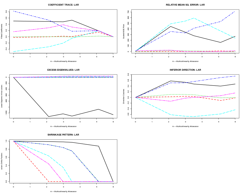
Details

RXuclars() applies Least Angle Regression to the uncorrelated components of a possibly ill-conditioned set of X-variables. A closed-form expression for the lars/lasso shrinkage delta factors exits in this case: Delta(i) = max(0,1-k/abs[PC(i)]), where PC(i) is the principal correlation between Y and the i-th principal coordinates of X. Note that the k-factor in this formulation is limited to a subset of [0,1]. MCAL=0 occurs at k=0, while MCAL = P results when k is the maximum absolute principal correlation.

Value

An output list object of class RXuclars:

`form`	The regression formula specified as the first argument.
`data`	Name of the data.frame object specified as the second argument.
`p`	Number of regression predictor variables.
`n`	Number of complete observations after removal of all missing values.
`r2`	Numerical value of R-square goodness-of-fit statistic.
`s2`	Numerical value of the residual mean square estimate of error.
`prinstat`	Listing of principal statistics.
`gmat`	Orthogonal matrix of direction cosines for regressor principal axes.
`lars`	An object of class lars.
`coef`	Matrix of shrinkage-ridge regression coefficient estimates.
`risk`	Matrix of MSE risk estimates for fitted coefficients.
`exev`	Matrix of excess MSE eigenvalues (ordinary least squares minus ridge.)
`infd`	Matrix of direction cosines for the estimated inferior direction, if any.
`spat`	Matrix of shrinkage pattern multiplicative delta factors.
`mlik`	Listing of criteria for maximum likelihood selection of M-extent-of-shrinkage.
`sext`	Listing of summary statistics for all M-extents-of-shrinkage.

Author(s)

Bob Obenchain <wizbob@att.net>

References

Efron B, Hastie T, Johnstone I, Tibshirani R. (2004) Least angle regression. Ann. Statis. 32, 407-499 (with discussion.)

Obenchain RL. (1994-2005) Shrinkage Regression: ridge, BLUP, Bayes, spline and Stein. members.iquest.net/~softrx.

Obenchain RL. (2011) shrink.PDF Vignette-like documentation stored in the R library/RXshrink/doc folder. 23 pages.

Examples

  data(longley2)
  form <- GNP~GNP.deflator+Unemployed+Armed.Forces+Population+Year+Employed
  rxuobj <- RXuclars(form, data=longley2)
  rxuobj
  plot(rxuobj)

Results


R version 3.3.1 (2016-06-21) -- "Bug in Your Hair"
Copyright (C) 2016 The R Foundation for Statistical Computing
Platform: x86_64-pc-linux-gnu (64-bit)

R is free software and comes with ABSOLUTELY NO WARRANTY.
You are welcome to redistribute it under certain conditions.
Type 'license()' or 'licence()' for distribution details.

R is a collaborative project with many contributors.
Type 'contributors()' for more information and
'citation()' on how to cite R or R packages in publications.

Type 'demo()' for some demos, 'help()' for on-line help, or
'help.start()' for an HTML browser interface to help.
Type 'q()' to quit R.

> library(RXshrink)
Loading required package: lars
Loaded lars 1.2

> png(filename="/home/ddbj/snapshot/RGM3/R_CC/result/RXshrink/RXuclars.Rd_%03d_medium.png", width=480, height=480)
> ### Name: RXuclars
> ### Title: Maximum Likelihood Least Angle Regression on Uncorrelated
> ###   X-Components
> ### Aliases: RXuclars
> ### Keywords: regression hplot
> 
> ### ** Examples
> 
>   data(longley2)
>   form <- GNP~GNP.deflator+Unemployed+Armed.Forces+Population+Year+Employed
>   rxuobj <- RXuclars(form, data=longley2)
>   rxuobj

RXuclars Object: Uncorrelated Component LARS Shrinkage
Data Frame: longley2 
Regression Equation:
GNP ~ GNP.deflator + Unemployed + Armed.Forces + Population + 
    Year + Employed

    Number of Regressor Variables, p = 6 
    Number of Observations, n = 29 

Principal Axis Summary Statistics of Ill-Conditioning...
        LAMBDA         SV         COMP         RHO       TRAT
1 124.55432117 11.1603907  0.466590166  0.98409260 179.451944
2  34.04395492  5.8347198 -0.009779055 -0.01078296  -1.966301
3   7.97601572  2.8241841  0.228918857  0.12217872  22.279619
4   1.31429584  1.1464274 -0.557948473 -0.12088200 -22.043160
5   0.06505309  0.2550551  0.613987118  0.02959472   5.396677
6   0.04635925  0.2153120 -0.471410409 -0.01918176  -3.497845

    Residual Mean Square for Error = 0.0008420418 
    Estimate of Residual Std. Error = 0.02901796 


The extent of shrinkage (M value) most likely to be optimal
depends upon whether one uses the Classical, Empirical Bayes, or
Random Coefficient criterion.  In each case, the objective is to
minimize the minus-two-log-likelihood statistics listed below:
         M     CLIK       EBAY     RCOF
0 0.000000      Inf        Inf      Inf
1 2.114916 149.4278   472.3079 100.5459
2 2.983319 157.4982   825.7711 113.6821
3 3.517121 164.6308  1259.1945 124.0563
4 5.112223 187.2225  4980.0349 159.4655
5 5.124154 187.5178  5027.7148 159.7195
6 6.000000 212.3044 33230.5079 212.3044

Extent of shrinkage statistics...
       TSMSE     MCAL
0   37.86637 0.000000
1 1330.28575 2.114916
2 1226.23804 2.983319
3 1296.89147 3.517121
4 1068.18888 5.112223
5 1069.64994 5.124154
6 1237.17669 6.000000

Output from LARS invocation...

Call:
lars(x = sx$u, y = cry, type = type, trace = trace, normalize = eps)
R-squared: 0.999 
Sequence of LAR moves:
                
Var  1 3 4 5 6 2
Step 1 2 3 4 5 6
>   plot(rxuobj)
> 
> 
> 
> 
> 
> dev.off()
null device 
          1 
>