R Graphical Manual

Browse All

Last data update: 2014.03.03

R: Attaches a Property to a Two-Dimensional Grid

setup.prop.2D

R Documentation

Attaches a Property to a Two-Dimensional Grid

Description

Calculates the value of a given property at the middle of grid cells (mid) and at the interfaces of the grid cells (int).

Two possibilities are available: either specifying a mathematical function (func) that describes the spatial dependency of the property, or asssuming a constant value (value). To allow for anisotropy, the spatial dependency can be different in the x and y direction.

For example, in a sediment model, the routine can be used to specify the porosity, the mixing intensity or other parameters over the grid of the reactangular sediment domain.

Usage

setup.prop.2D(func = NULL, value = NULL, grid, y.func = func, 
              y.value = value, ...)

## S3 method for class 'prop.2D'
contour(x, grid, xyswap = FALSE, filled = FALSE, ...)

Arguments

`func`	function that describes the spatial dependency in the x-direction; defined as `func <- function (x,y, ...); it should return as many elements as in x or y`
`value`	constant value given to the property in the x-direction
`grid`	list specifying the 2D grid characteristics, see `setup.grid.2D` for details on the structure of this list
`y.func`	function that describes the spatial dependency in the y-direction; defined as `y.func <- function (x, y, ...)`; it should return as many elements as in x or y. By default the same as in the x-direction.
`y.value`	constant value given to the property in the y-direction. By default the same as in the x-direction.
`x`	the object of class `prop.2D` that needs plotting
`filled`	if `TRUE`, uses `filled.contour`, else `contour`
`xyswap`	if `TRUE`, then x- and y-values are swapped and the y-axis is oriented from top to bottom. Useful for drawing vertical depth profiles
`...`	additional arguments that are passed on to `func` or to the method

Details

When the property is isotropic, the x.mid and y.mid values are identical. This is for example the case for sediment porosity.
When the property is anisotropic, the x.mid and y.mid values can differ. This can be for example the case for the velocity, where in general, the value will differ between the x and y direction.

Value

A list of type prop.2D containing:

`x.mid`	property value in the x-direction defined at the middle of the grid cells; Nx * Ny matrix (where Nx and Ny = number of cells in x, y direction)
`y.mid`	property value in the y-direction at the middle of the grid cells; Nx * Ny matrix
`x.int`	property value in the x-direction defined at the x-interfaces of the grid cells; (Nx+1)*Ny matrix
`y.int`	property value in the y-direction at the y-interfaces of the grid cells; Nx*(Ny+1) matrix

Note

For some properties, it does not make sense to use y.func different to func. For instance, for volume fractions, AFDW.

For other properties, it may be usefull to have y.func or y.value different from func or value, for instance for velocities, surface areas, ...

Author(s)

Filip Meysman <filip.meysman@nioz.nl>, Karline Soetaert <karline.soetaert@nioz.nl>

Examples

# Inverse quadratic function 
inv.quad <- function(x, y, a = NULL, b = NULL)
   return(1/((x-a)^2+(y-b)^2))


# Construction of the 2D grid 
x.grid <- setup.grid.1D (x.up = 0, L = 10, N = 10)
y.grid <- setup.grid.1D (x.up = 0, L = 10, N = 10)
grid2D <- setup.grid.2D (x.grid, y.grid)

# Attaching the inverse quadratic function to the 2D grid 
(twoD <- setup.prop.2D (func = inv.quad, grid = grid2D, a = 5, b = 5))

# show 
contour(log(twoD$x.int))

Results


R version 3.3.1 (2016-06-21) -- "Bug in Your Hair"
Copyright (C) 2016 The R Foundation for Statistical Computing
Platform: x86_64-pc-linux-gnu (64-bit)

R is free software and comes with ABSOLUTELY NO WARRANTY.
You are welcome to redistribute it under certain conditions.
Type 'license()' or 'licence()' for distribution details.

R is a collaborative project with many contributors.
Type 'contributors()' for more information and
'citation()' on how to cite R or R packages in publications.

Type 'demo()' for some demos, 'help()' for on-line help, or
'help.start()' for an HTML browser interface to help.
Type 'q()' to quit R.

> library(ReacTran)
Loading required package: rootSolve
Loading required package: deSolve

Attaching package: 'deSolve'

The following object is masked from 'package:graphics':

    matplot

Loading required package: shape
> png(filename="/home/ddbj/snapshot/RGM3/R_CC/result/ReacTran/setup.prop.2D.Rd_%03d_medium.png", width=480, height=480)
> ### Name: setup.prop.2D
> ### Title: Attaches a Property to a Two-Dimensional Grid
> ### Aliases: setup.prop.2D contour.prop.2D
> ### Keywords: utilities
> 
> ### ** Examples
> 
> # Inverse quadratic function 
> inv.quad <- function(x, y, a = NULL, b = NULL)
+    return(1/((x-a)^2+(y-b)^2))
> 
> 
> # Construction of the 2D grid 
> x.grid <- setup.grid.1D (x.up = 0, L = 10, N = 10)
> y.grid <- setup.grid.1D (x.up = 0, L = 10, N = 10)
> grid2D <- setup.grid.2D (x.grid, y.grid)
> 
> # Attaching the inverse quadratic function to the 2D grid 
> (twoD <- setup.prop.2D (func = inv.quad, grid = grid2D, a = 5, b = 5))
$x.mid
            [,1]       [,2]       [,3]       [,4]       [,5]       [,6]
 [1,] 0.02469136 0.03076923 0.03773585 0.04444444 0.04878049 0.04878049
 [2,] 0.03076923 0.04081633 0.05405405 0.06896552 0.08000000 0.08000000
 [3,] 0.03773585 0.05405405 0.08000000 0.11764706 0.15384615 0.15384615
 [4,] 0.04444444 0.06896552 0.11764706 0.22222222 0.40000000 0.40000000
 [5,] 0.04878049 0.08000000 0.15384615 0.40000000 2.00000000 2.00000000
 [6,] 0.04878049 0.08000000 0.15384615 0.40000000 2.00000000 2.00000000
 [7,] 0.04444444 0.06896552 0.11764706 0.22222222 0.40000000 0.40000000
 [8,] 0.03773585 0.05405405 0.08000000 0.11764706 0.15384615 0.15384615
 [9,] 0.03076923 0.04081633 0.05405405 0.06896552 0.08000000 0.08000000
[10,] 0.02469136 0.03076923 0.03773585 0.04444444 0.04878049 0.04878049
            [,7]       [,8]       [,9]      [,10]
 [1,] 0.04444444 0.03773585 0.03076923 0.02469136
 [2,] 0.06896552 0.05405405 0.04081633 0.03076923
 [3,] 0.11764706 0.08000000 0.05405405 0.03773585
 [4,] 0.22222222 0.11764706 0.06896552 0.04444444
 [5,] 0.40000000 0.15384615 0.08000000 0.04878049
 [6,] 0.40000000 0.15384615 0.08000000 0.04878049
 [7,] 0.22222222 0.11764706 0.06896552 0.04444444
 [8,] 0.11764706 0.08000000 0.05405405 0.03773585
 [9,] 0.06896552 0.05405405 0.04081633 0.03076923
[10,] 0.04444444 0.03773585 0.03076923 0.02469136

$y.mid
            [,1]       [,2]       [,3]       [,4]       [,5]       [,6]
 [1,] 0.02469136 0.03076923 0.03773585 0.04444444 0.04878049 0.04878049
 [2,] 0.03076923 0.04081633 0.05405405 0.06896552 0.08000000 0.08000000
 [3,] 0.03773585 0.05405405 0.08000000 0.11764706 0.15384615 0.15384615
 [4,] 0.04444444 0.06896552 0.11764706 0.22222222 0.40000000 0.40000000
 [5,] 0.04878049 0.08000000 0.15384615 0.40000000 2.00000000 2.00000000
 [6,] 0.04878049 0.08000000 0.15384615 0.40000000 2.00000000 2.00000000
 [7,] 0.04444444 0.06896552 0.11764706 0.22222222 0.40000000 0.40000000
 [8,] 0.03773585 0.05405405 0.08000000 0.11764706 0.15384615 0.15384615
 [9,] 0.03076923 0.04081633 0.05405405 0.06896552 0.08000000 0.08000000
[10,] 0.02469136 0.03076923 0.03773585 0.04444444 0.04878049 0.04878049
            [,7]       [,8]       [,9]      [,10]
 [1,] 0.04444444 0.03773585 0.03076923 0.02469136
 [2,] 0.06896552 0.05405405 0.04081633 0.03076923
 [3,] 0.11764706 0.08000000 0.05405405 0.03773585
 [4,] 0.22222222 0.11764706 0.06896552 0.04444444
 [5,] 0.40000000 0.15384615 0.08000000 0.04878049
 [6,] 0.40000000 0.15384615 0.08000000 0.04878049
 [7,] 0.22222222 0.11764706 0.06896552 0.04444444
 [8,] 0.11764706 0.08000000 0.05405405 0.03773585
 [9,] 0.06896552 0.05405405 0.04081633 0.03076923
[10,] 0.04444444 0.03773585 0.03076923 0.02469136

$x.int
            [,1]       [,2]       [,3]       [,4]       [,5]       [,6]
 [1,] 0.02209945 0.02684564 0.03200000 0.03669725 0.03960396 0.03960396
 [2,] 0.02758621 0.03539823 0.04494382 0.05479452 0.06153846 0.06153846
 [3,] 0.03418803 0.04705882 0.06557377 0.08888889 0.10810811 0.10810811
 [4,] 0.04123711 0.06153846 0.09756098 0.16000000 0.23529412 0.23529412
 [5,] 0.04705882 0.07547170 0.13793103 0.30769231 0.80000000 0.80000000
 [6,] 0.04938272 0.08163265 0.16000000 0.44444444 4.00000000 4.00000000
 [7,] 0.04705882 0.07547170 0.13793103 0.30769231 0.80000000 0.80000000
 [8,] 0.04123711 0.06153846 0.09756098 0.16000000 0.23529412 0.23529412
 [9,] 0.03418803 0.04705882 0.06557377 0.08888889 0.10810811 0.10810811
[10,] 0.02758621 0.03539823 0.04494382 0.05479452 0.06153846 0.06153846
[11,] 0.02209945 0.02684564 0.03200000 0.03669725 0.03960396 0.03960396
            [,7]       [,8]       [,9]      [,10]
 [1,] 0.03669725 0.03200000 0.02684564 0.02209945
 [2,] 0.05479452 0.04494382 0.03539823 0.02758621
 [3,] 0.08888889 0.06557377 0.04705882 0.03418803
 [4,] 0.16000000 0.09756098 0.06153846 0.04123711
 [5,] 0.30769231 0.13793103 0.07547170 0.04705882
 [6,] 0.44444444 0.16000000 0.08163265 0.04938272
 [7,] 0.30769231 0.13793103 0.07547170 0.04705882
 [8,] 0.16000000 0.09756098 0.06153846 0.04123711
 [9,] 0.08888889 0.06557377 0.04705882 0.03418803
[10,] 0.05479452 0.04494382 0.03539823 0.02758621
[11,] 0.03669725 0.03200000 0.02684564 0.02209945

$y.int
            [,1]       [,2]       [,3]       [,4]       [,5]       [,6]
 [1,] 0.02209945 0.02758621 0.03418803 0.04123711 0.04705882 0.04938272
 [2,] 0.02684564 0.03539823 0.04705882 0.06153846 0.07547170 0.08163265
 [3,] 0.03200000 0.04494382 0.06557377 0.09756098 0.13793103 0.16000000
 [4,] 0.03669725 0.05479452 0.08888889 0.16000000 0.30769231 0.44444444
 [5,] 0.03960396 0.06153846 0.10810811 0.23529412 0.80000000 4.00000000
 [6,] 0.03960396 0.06153846 0.10810811 0.23529412 0.80000000 4.00000000
 [7,] 0.03669725 0.05479452 0.08888889 0.16000000 0.30769231 0.44444444
 [8,] 0.03200000 0.04494382 0.06557377 0.09756098 0.13793103 0.16000000
 [9,] 0.02684564 0.03539823 0.04705882 0.06153846 0.07547170 0.08163265
[10,] 0.02209945 0.02758621 0.03418803 0.04123711 0.04705882 0.04938272
            [,7]       [,8]       [,9]      [,10]      [,11]
 [1,] 0.04705882 0.04123711 0.03418803 0.02758621 0.02209945
 [2,] 0.07547170 0.06153846 0.04705882 0.03539823 0.02684564
 [3,] 0.13793103 0.09756098 0.06557377 0.04494382 0.03200000
 [4,] 0.30769231 0.16000000 0.08888889 0.05479452 0.03669725
 [5,] 0.80000000 0.23529412 0.10810811 0.06153846 0.03960396
 [6,] 0.80000000 0.23529412 0.10810811 0.06153846 0.03960396
 [7,] 0.30769231 0.16000000 0.08888889 0.05479452 0.03669725
 [8,] 0.13793103 0.09756098 0.06557377 0.04494382 0.03200000
 [9,] 0.07547170 0.06153846 0.04705882 0.03539823 0.02684564
[10,] 0.04705882 0.04123711 0.03418803 0.02758621 0.02209945

attr(,"class")
[1] "prop.2D"
> 
> # show 
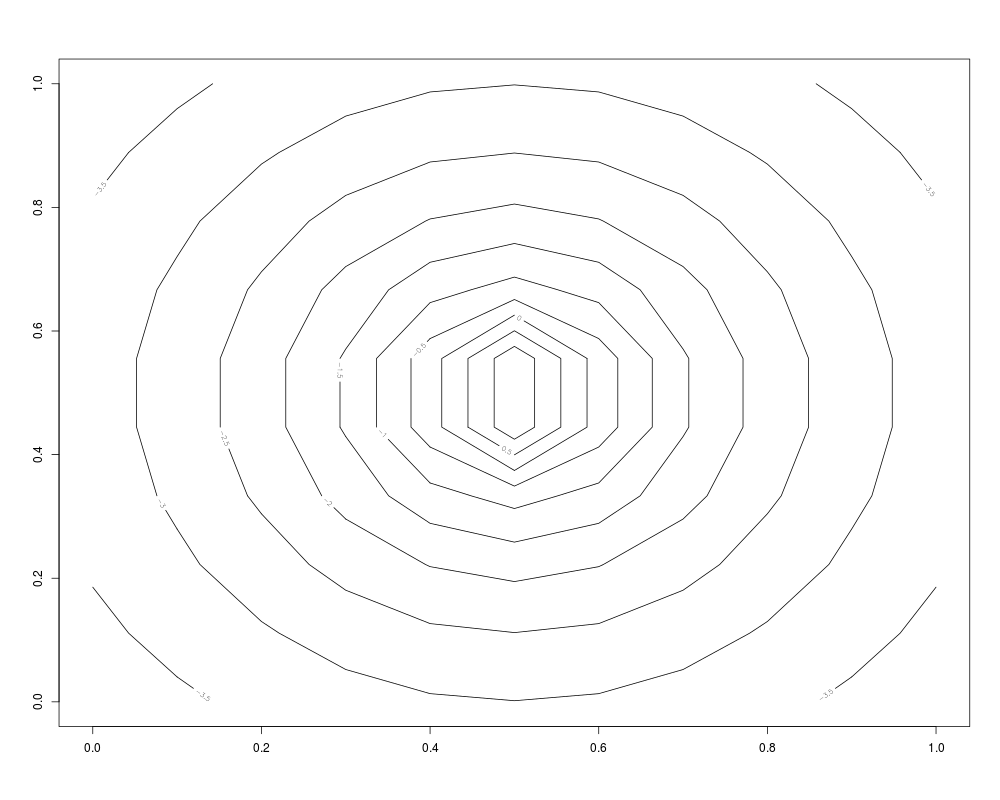
> contour(log(twoD$x.int))
> 
> 
> 
> 
> 
> 
> dev.off()
null device 
          1 
>