Supported by Dr. Osamu Ogasawara and  . . |
|
Last data update: 2014.03.03 |
Hierarchical Modeling and Frequency Method Checking on Overdispersed Gaussian, Poisson, and Binomial DataDescriptionBayesian-frequentist reconciliation via approximate Bayesian hierarchical modeling and frequency method checking for over-dispersed Gaussian, Binomial, and Poisson data. Details
Author(s)Hyungsuk Tak, Joseph Kelly, and Carl Morris Maintainer: Joseph Kelly <josephkelly@google.com> ReferencesMorris, C. and Lysy, M. (2012). Shrinkage Estimation in Multilevel Normal Models. Statistical Science. 27. 115-134. Examples
# Loading datasets
data(schools)
y <- schools$y
se <- schools$se
# Arbitrary covariate for schools data
x2 <- rep(c(-1, 0, 1, 2), 2)
# baseball data where z is Hits and n is AtBats
z <- c(18, 17, 16, 15, 14, 14, 13, 12, 11, 11, 10, 10, 10, 10, 10, 9, 8, 7)
n <- c(45, 45, 45, 45, 45, 45, 45, 45, 45, 45, 45, 45, 45, 45, 45, 45, 45, 45)
# One covariate: 1 if a player is an outfielder and 0 otherwise
x1 <- c(1, 1, 1, 1, 1, 0, 0, 0, 0, 1, 0, 0, 0, 1, 1, 0, 0, 0)
################################################################
# Gaussian Regression Interactive Multilevel Modeling (GRIMM) #
################################################################
####################################################################################
# If we do not have any covariate and do not know a mean of the prior distribution #
####################################################################################
g <- gbp(y, se, model = "gaussian")
g
print(g, sort = FALSE)
summary(g)
plot(g)
plot(g, sort = FALSE)
### when we want to simulate pseudo datasets considering the estimated values
### as true ones.
### gcv <- coverage(g, nsim = 10)
### more details in ?coverage
##################################################################################
# If we have one covariate and do not know a mean of the prior distribution yet, #
##################################################################################
g <- gbp(y, se, x2, model = "gaussian")
g
print(g, sort = FALSE)
summary(g)
plot(g)
plot(g, sort = FALSE)
### when we want to simulate pseudo datasets considering the estimated values
### as true ones.
### gcv <- coverage(g, nsim = 10)
### more details in ?coverage
################################################
# If we know a mean of the prior distribution, #
################################################
g <- gbp(y, se, mean.PriorDist = 8, model = "gaussian")
g
print(g, sort = FALSE)
summary(g)
plot(g)
plot(g, sort = FALSE)
### when we want to simulate pseudo datasets considering the estimated values
### as true ones.
### gcv <- coverage(g, nsim = 10)
### more details in ?coverage
###############################################################
# Binomial Regression Interactive Multilevel Modeling (BRIMM) #
###############################################################
####################################################################################
# If we do not have any covariate and do not know a mean of the prior distribution #
####################################################################################
b <- gbp(z, n, model = "binomial")
b
print(b, sort = FALSE)
summary(b)
plot(b)
plot(b, sort = FALSE)
### when we want to simulate pseudo datasets considering the estimated values
### as true ones.
### bcv <- coverage(b, nsim = 10)
### more details in ?coverage
##################################################################################
# If we have one covariate and do not know a mean of the prior distribution yet, #
##################################################################################
b <- gbp(z, n, x1, model = "binomial")
b
print(b, sort = FALSE)
summary(b)
plot(b)
plot(b, sort = FALSE)
### when we want to simulate pseudo datasets considering the estimated values
### as true ones.
### bcv <- coverage(b, nsim = 10)
### more details in ?coverage
################################################
# If we know a mean of the prior distribution, #
################################################
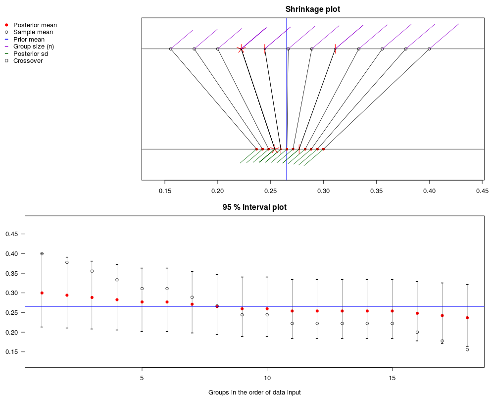
b <- gbp(z, n, mean.PriorDist = 0.265, model = "binomial")
b
print(b, sort = FALSE)
summary(b)
plot(b)
plot(b, sort = FALSE)
### when we want to simulate pseudo datasets considering the estimated values
### as true ones.
### bcv <- coverage(b, nsim = 10)
### more details in ?coverage
##############################################################
# Poisson Regression Interactive Multilevel Modeling (PRIMM) #
##############################################################
################################################
# If we know a mean of the prior distribution, #
################################################
p <- gbp(z, n, mean.PriorDist = 0.265, model = "poisson")
p
print(p, sort = FALSE)
summary(p)
plot(p)
plot(p, sort = FALSE)
### when we want to simulate pseudo datasets considering the estimated values
### as true ones.
### pcv <- coverage(p, nsim = 10)
### more details in ?coverage
Results
R version 3.3.1 (2016-06-21) -- "Bug in Your Hair"
Copyright (C) 2016 The R Foundation for Statistical Computing
Platform: x86_64-pc-linux-gnu (64-bit)
R is free software and comes with ABSOLUTELY NO WARRANTY.
You are welcome to redistribute it under certain conditions.
Type 'license()' or 'licence()' for distribution details.
R is a collaborative project with many contributors.
Type 'contributors()' for more information and
'citation()' on how to cite R or R packages in publications.
Type 'demo()' for some demos, 'help()' for on-line help, or
'help.start()' for an HTML browser interface to help.
Type 'q()' to quit R.
> library(Rgbp)
Loading required package: sn
Loading required package: stats4
Attaching package: 'sn'
The following object is masked from 'package:stats':
sd
Loading required package: mnormt
> png(filename="/home/ddbj/snapshot/RGM3/R_CC/result/Rgbp/Rgbp-package.Rd_%03d_medium.png", width=480, height=480)
> ### Name: Rgbp
> ### Title: Hierarchical Modeling and Frequency Method Checking on
> ### Overdispersed Gaussian, Poisson, and Binomial Data
> ### Aliases: Rgbp-package Rgbp
> ### Keywords: package
>
> ### ** Examples
>
>
> # Loading datasets
> data(schools)
> y <- schools$y
> se <- schools$se
>
> # Arbitrary covariate for schools data
> x2 <- rep(c(-1, 0, 1, 2), 2)
>
> # baseball data where z is Hits and n is AtBats
> z <- c(18, 17, 16, 15, 14, 14, 13, 12, 11, 11, 10, 10, 10, 10, 10, 9, 8, 7)
> n <- c(45, 45, 45, 45, 45, 45, 45, 45, 45, 45, 45, 45, 45, 45, 45, 45, 45, 45)
>
> # One covariate: 1 if a player is an outfielder and 0 otherwise
> x1 <- c(1, 1, 1, 1, 1, 0, 0, 0, 0, 1, 0, 0, 0, 1, 1, 0, 0, 0)
>
> ################################################################
> # Gaussian Regression Interactive Multilevel Modeling (GRIMM) #
> ################################################################
>
> ####################################################################################
> # If we do not have any covariate and do not know a mean of the prior distribution #
> ####################################################################################
>
> g <- gbp(y, se, model = "gaussian")
> g
Summary for each group (sorted by the descending order of se):
obs.mean se prior.mean shrinkage low.intv post.mean upp.intv post.sd
8 12.00 18.0 8.17 0.734 -10.21 9.19 29.9 10.23
3 -3.00 16.0 8.17 0.685 -17.13 4.65 22.5 10.10
1 28.00 15.0 8.17 0.657 -2.32 14.98 38.8 10.56
4 7.00 11.0 8.17 0.507 -8.78 7.59 23.6 8.26
6 1.00 11.0 8.17 0.507 -13.03 4.63 20.1 8.44
2 8.00 10.0 8.17 0.459 -7.25 8.08 23.4 7.81
7 18.00 10.0 8.17 0.459 -1.29 13.48 30.8 8.18
5 -1.00 9.0 8.17 0.408 -13.30 2.74 16.7 7.63
Mean 12.5 8.17 0.552 -9.16 8.17 25.7 8.90
> print(g, sort = FALSE)
Summary for each group:
obs.mean se prior.mean shrinkage low.intv post.mean upp.intv post.sd
1 28.00 15.0 8.17 0.657 -2.32 14.98 38.8 10.56
2 8.00 10.0 8.17 0.459 -7.25 8.08 23.4 7.81
3 -3.00 16.0 8.17 0.685 -17.13 4.65 22.5 10.10
4 7.00 11.0 8.17 0.507 -8.78 7.59 23.6 8.26
5 -1.00 9.0 8.17 0.408 -13.30 2.74 16.7 7.63
6 1.00 11.0 8.17 0.507 -13.03 4.63 20.1 8.44
7 18.00 10.0 8.17 0.459 -1.29 13.48 30.8 8.18
8 12.00 18.0 8.17 0.734 -10.21 9.19 29.9 10.23
Mean 12.5 8.17 0.552 -9.16 8.17 25.7 8.90
> summary(g)
Main summary:
obs.mean se prior.mean shrinkage low.intv post.mean
Group with min(se) -1.00 9.0 8.17 0.408 -13.30 2.74
Group with median(se)1 1.00 11.0 8.17 0.507 -13.03 4.63
Group with median(se)2 7.00 11.0 8.17 0.507 -8.78 7.59
Group with max(se) 12.00 18.0 8.17 0.734 -10.21 9.19
Overall Mean 12.5 8.17 0.552 -9.16 8.17
upp.intv post.sd
Group with min(se) 16.7 7.63
Group with median(se)1 20.1 8.44
Group with median(se)2 23.6 8.26
Group with max(se) 29.9 10.23
Overall Mean 25.7 8.90
Estimation summary for the second-level variance component:
alpha = log(A) for Gaussian or alpha = log(1/r) for Binomial and Poisson data:
post.mode.alpha post.sd.alpha post.mode.A
4.77 1.14 118
Estimation summary for the regression coefficient :
estimate se z.val p.val
beta1 8.168 5.73 1.425 0.154
> plot(g)
> plot(g, sort = FALSE)
>
> ### when we want to simulate pseudo datasets considering the estimated values
> ### as true ones.
> ### gcv <- coverage(g, nsim = 10)
> ### more details in ?coverage
>
> ##################################################################################
> # If we have one covariate and do not know a mean of the prior distribution yet, #
> ##################################################################################
>
> g <- gbp(y, se, x2, model = "gaussian")
> g
Summary for each group (sorted by the descending order of se):
obs.mean se X1 prior.mean shrinkage low.intv post.mean upp.intv
8 12.00 18.0 2.0 8.45 0.666 -14.83 9.64 35.2
3 -3.00 16.0 1.0 8.32 0.612 -20.05 3.93 23.9
1 28.00 15.0 -1.0 8.07 0.581 -5.14 16.43 43.4
4 7.00 11.0 2.0 8.45 0.427 -11.30 7.62 26.2
6 1.00 11.0 0.0 8.20 0.427 -14.51 4.07 20.8
2 8.00 10.0 0.0 8.20 0.381 -8.15 8.08 24.3
7 18.00 10.0 1.0 8.32 0.381 -1.59 14.31 32.3
5 -1.00 9.0 -1.0 8.07 0.333 -15.14 2.02 17.7
Mean 12.5 0.5 8.26 0.476 -11.34 8.26 28.0
post.sd
8 12.74
3 11.20
1 12.39
4 9.56
6 8.98
2 8.27
7 8.63
5 8.35
Mean 10.02
> print(g, sort = FALSE)
Summary for each group:
obs.mean se X1 prior.mean shrinkage low.intv post.mean upp.intv
1 28.00 15.0 -1.0 8.07 0.581 -5.14 16.43 43.4
2 8.00 10.0 0.0 8.20 0.381 -8.15 8.08 24.3
3 -3.00 16.0 1.0 8.32 0.612 -20.05 3.93 23.9
4 7.00 11.0 2.0 8.45 0.427 -11.30 7.62 26.2
5 -1.00 9.0 -1.0 8.07 0.333 -15.14 2.02 17.7
6 1.00 11.0 0.0 8.20 0.427 -14.51 4.07 20.8
7 18.00 10.0 1.0 8.32 0.381 -1.59 14.31 32.3
8 12.00 18.0 2.0 8.45 0.666 -14.83 9.64 35.2
Mean 12.5 0.5 8.26 0.476 -11.34 8.26 28.0
post.sd
1 12.39
2 8.27
3 11.20
4 9.56
5 8.35
6 8.98
7 8.63
8 12.74
Mean 10.02
> summary(g)
Main summary:
obs.mean se X1 prior.mean shrinkage low.intv
Group with min(se) -1.00 9.0 -1.0 8.07 0.333 -15.1
Group with median(se)1 1.00 11.0 0.0 8.20 0.427 -14.5
Group with median(se)2 7.00 11.0 2.0 8.45 0.427 -11.3
Group with max(se) 12.00 18.0 2.0 8.45 0.666 -14.8
Overall Mean 12.5 0.5 8.26 0.476 -11.3
post.mean upp.intv post.sd
Group with min(se) 2.02 17.7 8.35
Group with median(se)1 4.07 20.8 8.98
Group with median(se)2 7.62 26.2 9.56
Group with max(se) 9.64 35.2 12.74
Overall Mean 8.26 28.0 10.02
Estimation summary for the second-level variance component:
alpha = log(A) for Gaussian or alpha = log(1/r) for Binomial and Poisson data:
post.mode.alpha post.sd.alpha post.mode.A
5.09 1.17 162
Estimation summary for the regression coefficient :
estimate se z.val p.val
beta1 8.198 6.656 1.232 0.218
beta2 0.126 5.698 0.022 0.982
> plot(g)
> plot(g, sort = FALSE)
>
> ### when we want to simulate pseudo datasets considering the estimated values
> ### as true ones.
> ### gcv <- coverage(g, nsim = 10)
> ### more details in ?coverage
>
> ################################################
> # If we know a mean of the prior distribution, #
> ################################################
>
> g <- gbp(y, se, mean.PriorDist = 8, model = "gaussian")
> g
Summary for each group (sorted by the descending order of se):
obs.mean se prior.mean shrinkage low.intv post.mean upp.intv post.sd
8 12.00 18.0 8 0.786 -6.767 8.86 26.1 8.36
3 -3.00 16.0 8 0.743 -13.448 5.18 19.3 8.38
1 28.00 15.0 8 0.718 0.595 13.64 34.6 8.95
4 7.00 11.0 8 0.578 -6.642 7.58 21.4 7.15
6 1.00 11.0 8 0.578 -10.701 5.04 18.1 7.34
2 8.00 10.0 8 0.531 -5.426 8.00 21.4 6.85
7 18.00 10.0 8 0.531 0.123 12.69 28.6 7.27
5 -1.00 9.0 8 0.478 -11.516 3.30 15.4 6.87
Mean 12.5 8 0.618 -6.723 8.04 23.1 7.65
> print(g, sort = FALSE)
Summary for each group:
obs.mean se prior.mean shrinkage low.intv post.mean upp.intv post.sd
1 28.00 15.0 8 0.718 0.595 13.64 34.6 8.95
2 8.00 10.0 8 0.531 -5.426 8.00 21.4 6.85
3 -3.00 16.0 8 0.743 -13.448 5.18 19.3 8.38
4 7.00 11.0 8 0.578 -6.642 7.58 21.4 7.15
5 -1.00 9.0 8 0.478 -11.516 3.30 15.4 6.87
6 1.00 11.0 8 0.578 -10.701 5.04 18.1 7.34
7 18.00 10.0 8 0.531 0.123 12.69 28.6 7.27
8 12.00 18.0 8 0.786 -6.767 8.86 26.1 8.36
Mean 12.5 8 0.618 -6.723 8.04 23.1 7.65
> summary(g)
Main summary:
obs.mean se prior.mean shrinkage low.intv post.mean
Group with min(se) -1.00 9.0 8 0.478 -11.52 3.30
Group with median(se)1 1.00 11.0 8 0.578 -10.70 5.04
Group with median(se)2 7.00 11.0 8 0.578 -6.64 7.58
Group with max(se) 12.00 18.0 8 0.786 -6.77 8.86
Overall Mean 12.5 8 0.618 -6.72 8.04
upp.intv post.sd
Group with min(se) 15.4 6.87
Group with median(se)1 18.1 7.34
Group with median(se)2 21.4 7.15
Group with max(se) 26.1 8.36
Overall Mean 23.1 7.65
Estimation summary for the second-level variance component:
alpha = log(A) for Gaussian or alpha = log(1/r) for Binomial and Poisson data:
post.mode.alpha post.sd.alpha post.mode.A
4.48 1.13 88.4
> plot(g)
> plot(g, sort = FALSE)
>
> ### when we want to simulate pseudo datasets considering the estimated values
> ### as true ones.
> ### gcv <- coverage(g, nsim = 10)
> ### more details in ?coverage
>
> ###############################################################
> # Binomial Regression Interactive Multilevel Modeling (BRIMM) #
> ###############################################################
>
> ####################################################################################
> # If we do not have any covariate and do not know a mean of the prior distribution #
> ####################################################################################
>
> b <- gbp(z, n, model = "binomial")
> b
Summary for each group (sorted by the ascending order of n):
obs.mean n prior.mean shrinkage low.intv post.mean upp.intv post.sd
1 0.400 45 0.267 0.622 0.222 0.317 0.421 0.0507
2 0.378 45 0.267 0.622 0.218 0.309 0.408 0.0487
3 0.356 45 0.267 0.622 0.213 0.300 0.396 0.0469
4 0.333 45 0.267 0.622 0.207 0.292 0.385 0.0453
5 0.311 45 0.267 0.622 0.202 0.284 0.374 0.0440
6 0.311 45 0.267 0.622 0.202 0.284 0.374 0.0440
7 0.289 45 0.267 0.622 0.195 0.275 0.363 0.0431
8 0.267 45 0.267 0.622 0.188 0.267 0.354 0.0424
9 0.244 45 0.267 0.622 0.180 0.258 0.345 0.0421
10 0.244 45 0.267 0.622 0.180 0.258 0.345 0.0421
11 0.222 45 0.267 0.622 0.172 0.250 0.337 0.0422
12 0.222 45 0.267 0.622 0.172 0.250 0.337 0.0422
13 0.222 45 0.267 0.622 0.172 0.250 0.337 0.0422
14 0.222 45 0.267 0.622 0.172 0.250 0.337 0.0422
15 0.222 45 0.267 0.622 0.172 0.250 0.337 0.0422
16 0.200 45 0.267 0.622 0.163 0.242 0.330 0.0426
17 0.178 45 0.267 0.622 0.154 0.233 0.323 0.0433
18 0.156 45 0.267 0.622 0.144 0.225 0.318 0.0444
Mean 45 0.267 0.622 0.185 0.266 0.357 0.0439
> print(b, sort = FALSE)
Summary for each group:
obs.mean n prior.mean shrinkage low.intv post.mean upp.intv post.sd
1 0.400 45 0.267 0.622 0.222 0.317 0.421 0.0507
2 0.378 45 0.267 0.622 0.218 0.309 0.408 0.0487
3 0.356 45 0.267 0.622 0.213 0.300 0.396 0.0469
4 0.333 45 0.267 0.622 0.207 0.292 0.385 0.0453
5 0.311 45 0.267 0.622 0.202 0.284 0.374 0.0440
6 0.311 45 0.267 0.622 0.202 0.284 0.374 0.0440
7 0.289 45 0.267 0.622 0.195 0.275 0.363 0.0431
8 0.267 45 0.267 0.622 0.188 0.267 0.354 0.0424
9 0.244 45 0.267 0.622 0.180 0.258 0.345 0.0421
10 0.244 45 0.267 0.622 0.180 0.258 0.345 0.0421
11 0.222 45 0.267 0.622 0.172 0.250 0.337 0.0422
12 0.222 45 0.267 0.622 0.172 0.250 0.337 0.0422
13 0.222 45 0.267 0.622 0.172 0.250 0.337 0.0422
14 0.222 45 0.267 0.622 0.172 0.250 0.337 0.0422
15 0.222 45 0.267 0.622 0.172 0.250 0.337 0.0422
16 0.200 45 0.267 0.622 0.163 0.242 0.330 0.0426
17 0.178 45 0.267 0.622 0.154 0.233 0.323 0.0433
18 0.156 45 0.267 0.622 0.144 0.225 0.318 0.0444
Mean 45 0.267 0.622 0.185 0.266 0.357 0.0439
> summary(b)
Main summary:
obs.mean n prior.mean shrinkage low.intv
Group with min(obs.mean) 0.156 45 0.267 0.622 0.144
Group with median(obs.mean)1 0.244 45 0.267 0.622 0.180
Group with median(obs.mean)2 0.244 45 0.267 0.622 0.180
Group with max(obs.mean) 0.400 45 0.267 0.622 0.222
Overall Mean 45 0.267 0.622 0.185
post.mean upp.intv post.sd
Group with min(obs.mean) 0.225 0.318 0.0444
Group with median(obs.mean)1 0.258 0.345 0.0421
Group with median(obs.mean)2 0.258 0.345 0.0421
Group with max(obs.mean) 0.317 0.421 0.0507
Overall Mean 0.266 0.357 0.0439
Estimation summary for the second-level variance component:
alpha = log(A) for Gaussian or alpha = log(1/r) for Binomial and Poisson data:
post.mode.alpha post.sd.alpha post.mode.r
-4.31 0.82 74.1
Estimation summary for the regression coefficient :
estimate se z.val p.val
beta1 -1.012 0.1 -10.153 0
> plot(b)
> plot(b, sort = FALSE)
>
> ### when we want to simulate pseudo datasets considering the estimated values
> ### as true ones.
> ### bcv <- coverage(b, nsim = 10)
> ### more details in ?coverage
>
> ##################################################################################
> # If we have one covariate and do not know a mean of the prior distribution yet, #
> ##################################################################################
>
> b <- gbp(z, n, x1, model = "binomial")
> b
Summary for each group (sorted by the ascending order of n):
obs.mean n X1 prior.mean shrinkage low.intv post.mean upp.intv post.sd
1 0.400 45 1.00 0.310 0.715 0.248 0.335 0.429 0.0462
2 0.378 45 1.00 0.310 0.715 0.244 0.329 0.420 0.0448
3 0.356 45 1.00 0.310 0.715 0.240 0.323 0.411 0.0437
4 0.333 45 1.00 0.310 0.715 0.236 0.316 0.403 0.0429
5 0.311 45 1.00 0.310 0.715 0.230 0.310 0.396 0.0424
6 0.311 45 0.00 0.233 0.715 0.179 0.256 0.341 0.0415
7 0.289 45 0.00 0.233 0.715 0.175 0.249 0.331 0.0400
8 0.267 45 0.00 0.233 0.715 0.171 0.243 0.323 0.0388
9 0.244 45 0.00 0.233 0.715 0.166 0.237 0.315 0.0380
10 0.244 45 1.00 0.310 0.715 0.210 0.291 0.379 0.0432
11 0.222 45 0.00 0.233 0.715 0.161 0.230 0.308 0.0377
12 0.222 45 0.00 0.233 0.715 0.161 0.230 0.308 0.0377
13 0.222 45 0.00 0.233 0.715 0.161 0.230 0.308 0.0377
14 0.222 45 1.00 0.310 0.715 0.202 0.285 0.375 0.0441
15 0.222 45 1.00 0.310 0.715 0.202 0.285 0.375 0.0441
16 0.200 45 0.00 0.233 0.715 0.155 0.224 0.302 0.0377
17 0.178 45 0.00 0.233 0.715 0.148 0.218 0.297 0.0381
18 0.156 45 0.00 0.233 0.715 0.140 0.211 0.292 0.0389
Mean 45 0.44 0.267 0.715 0.191 0.267 0.351 0.0410
> print(b, sort = FALSE)
Summary for each group:
obs.mean n X1 prior.mean shrinkage low.intv post.mean upp.intv post.sd
1 0.400 45 1.00 0.310 0.715 0.248 0.335 0.429 0.0462
2 0.378 45 1.00 0.310 0.715 0.244 0.329 0.420 0.0448
3 0.356 45 1.00 0.310 0.715 0.240 0.323 0.411 0.0437
4 0.333 45 1.00 0.310 0.715 0.236 0.316 0.403 0.0429
5 0.311 45 1.00 0.310 0.715 0.230 0.310 0.396 0.0424
6 0.311 45 0.00 0.233 0.715 0.179 0.256 0.341 0.0415
7 0.289 45 0.00 0.233 0.715 0.175 0.249 0.331 0.0400
8 0.267 45 0.00 0.233 0.715 0.171 0.243 0.323 0.0388
9 0.244 45 0.00 0.233 0.715 0.166 0.237 0.315 0.0380
10 0.244 45 1.00 0.310 0.715 0.210 0.291 0.379 0.0432
11 0.222 45 0.00 0.233 0.715 0.161 0.230 0.308 0.0377
12 0.222 45 0.00 0.233 0.715 0.161 0.230 0.308 0.0377
13 0.222 45 0.00 0.233 0.715 0.161 0.230 0.308 0.0377
14 0.222 45 1.00 0.310 0.715 0.202 0.285 0.375 0.0441
15 0.222 45 1.00 0.310 0.715 0.202 0.285 0.375 0.0441
16 0.200 45 0.00 0.233 0.715 0.155 0.224 0.302 0.0377
17 0.178 45 0.00 0.233 0.715 0.148 0.218 0.297 0.0381
18 0.156 45 0.00 0.233 0.715 0.140 0.211 0.292 0.0389
Mean 45 0.44 0.267 0.715 0.191 0.267 0.351 0.0410
> summary(b)
Main summary:
obs.mean n X1 prior.mean shrinkage low.intv
Group with min(obs.mean) 0.156 45 0.000 0.233 0.715 0.140
Group with median(obs.mean)1 0.244 45 0.000 0.233 0.715 0.166
Group with median(obs.mean)2 0.244 45 1.000 0.310 0.715 0.210
Group with max(obs.mean) 0.400 45 1.000 0.310 0.715 0.248
Overall Mean 45 0.444 0.267 0.715 0.191
post.mean upp.intv post.sd
Group with min(obs.mean) 0.211 0.292 0.0389
Group with median(obs.mean)1 0.237 0.315 0.0380
Group with median(obs.mean)2 0.291 0.379 0.0432
Group with max(obs.mean) 0.335 0.429 0.0462
Overall Mean 0.267 0.351 0.0410
Estimation summary for the second-level variance component:
alpha = log(A) for Gaussian or alpha = log(1/r) for Binomial and Poisson data:
post.mode.alpha post.sd.alpha post.mode.r
-4.73 0.957 113
Estimation summary for the regression coefficient :
estimate se z.val p.val
beta1 -1.194 0.131 -9.129 0.000
beta2 0.389 0.187 2.074 0.038
> plot(b)
> plot(b, sort = FALSE)
>
> ### when we want to simulate pseudo datasets considering the estimated values
> ### as true ones.
> ### bcv <- coverage(b, nsim = 10)
> ### more details in ?coverage
>
> ################################################
> # If we know a mean of the prior distribution, #
> ################################################
>
> b <- gbp(z, n, mean.PriorDist = 0.265, model = "binomial")
> b
Summary for each group (sorted by the ascending order of n):
obs.mean n prior.mean shrinkage low.intv post.mean upp.intv post.sd
1 0.400 45 0.265 0.65 0.230 0.312 0.401 0.0439
2 0.378 45 0.265 0.65 0.224 0.304 0.391 0.0428
3 0.356 45 0.265 0.65 0.218 0.297 0.382 0.0418
4 0.333 45 0.265 0.65 0.212 0.289 0.372 0.0409
5 0.311 45 0.265 0.65 0.206 0.281 0.363 0.0401
6 0.311 45 0.265 0.65 0.206 0.281 0.363 0.0401
7 0.289 45 0.265 0.65 0.200 0.273 0.354 0.0395
8 0.267 45 0.265 0.65 0.193 0.266 0.345 0.0390
9 0.244 45 0.265 0.65 0.186 0.258 0.337 0.0386
10 0.244 45 0.265 0.65 0.186 0.258 0.337 0.0386
11 0.222 45 0.265 0.65 0.179 0.250 0.329 0.0383
12 0.222 45 0.265 0.65 0.179 0.250 0.329 0.0383
13 0.222 45 0.265 0.65 0.179 0.250 0.329 0.0383
14 0.222 45 0.265 0.65 0.179 0.250 0.329 0.0383
15 0.222 45 0.265 0.65 0.179 0.250 0.329 0.0383
16 0.200 45 0.265 0.65 0.172 0.242 0.321 0.0381
17 0.178 45 0.265 0.65 0.164 0.234 0.313 0.0381
18 0.156 45 0.265 0.65 0.156 0.227 0.306 0.0383
Mean 45 0.265 0.65 0.191 0.265 0.346 0.0395
> print(b, sort = FALSE)
Summary for each group:
obs.mean n prior.mean shrinkage low.intv post.mean upp.intv post.sd
1 0.400 45 0.265 0.65 0.230 0.312 0.401 0.0439
2 0.378 45 0.265 0.65 0.224 0.304 0.391 0.0428
3 0.356 45 0.265 0.65 0.218 0.297 0.382 0.0418
4 0.333 45 0.265 0.65 0.212 0.289 0.372 0.0409
5 0.311 45 0.265 0.65 0.206 0.281 0.363 0.0401
6 0.311 45 0.265 0.65 0.206 0.281 0.363 0.0401
7 0.289 45 0.265 0.65 0.200 0.273 0.354 0.0395
8 0.267 45 0.265 0.65 0.193 0.266 0.345 0.0390
9 0.244 45 0.265 0.65 0.186 0.258 0.337 0.0386
10 0.244 45 0.265 0.65 0.186 0.258 0.337 0.0386
11 0.222 45 0.265 0.65 0.179 0.250 0.329 0.0383
12 0.222 45 0.265 0.65 0.179 0.250 0.329 0.0383
13 0.222 45 0.265 0.65 0.179 0.250 0.329 0.0383
14 0.222 45 0.265 0.65 0.179 0.250 0.329 0.0383
15 0.222 45 0.265 0.65 0.179 0.250 0.329 0.0383
16 0.200 45 0.265 0.65 0.172 0.242 0.321 0.0381
17 0.178 45 0.265 0.65 0.164 0.234 0.313 0.0381
18 0.156 45 0.265 0.65 0.156 0.227 0.306 0.0383
Mean 45 0.265 0.65 0.191 0.265 0.346 0.0395
> summary(b)
Main summary:
obs.mean n prior.mean shrinkage low.intv
Group with min(obs.mean) 0.156 45 0.265 0.65 0.156
Group with median(obs.mean)1 0.244 45 0.265 0.65 0.186
Group with median(obs.mean)2 0.244 45 0.265 0.65 0.186
Group with max(obs.mean) 0.400 45 0.265 0.65 0.230
Overall Mean 45 0.265 0.65 0.191
post.mean upp.intv post.sd
Group with min(obs.mean) 0.227 0.306 0.0383
Group with median(obs.mean)1 0.258 0.337 0.0386
Group with median(obs.mean)2 0.258 0.337 0.0386
Group with max(obs.mean) 0.312 0.401 0.0439
Overall Mean 0.265 0.346 0.0395
Estimation summary for the second-level variance component:
alpha = log(A) for Gaussian or alpha = log(1/r) for Binomial and Poisson data:
post.mode.alpha post.sd.alpha post.mode.r
-4.42 0.837 83.5
> plot(b)
> plot(b, sort = FALSE)
>
> ### when we want to simulate pseudo datasets considering the estimated values
> ### as true ones.
> ### bcv <- coverage(b, nsim = 10)
> ### more details in ?coverage
>
> ##############################################################
> # Poisson Regression Interactive Multilevel Modeling (PRIMM) #
> ##############################################################
>
> ################################################
> # If we know a mean of the prior distribution, #
> ################################################
>
> p <- gbp(z, n, mean.PriorDist = 0.265, model = "poisson")
> p
Summary for each group (sorted by the ascending order of n):
obs.mean n prior.mean shrinkage low.intv post.mean upp.intv post.sd
1 0.400 45 0.265 0.741 0.213 0.300 0.402 0.0483
2 0.378 45 0.265 0.741 0.211 0.294 0.391 0.0461
3 0.356 45 0.265 0.741 0.208 0.288 0.381 0.0442
4 0.333 45 0.265 0.741 0.206 0.283 0.372 0.0424
5 0.311 45 0.265 0.741 0.202 0.277 0.363 0.0410
6 0.311 45 0.265 0.741 0.202 0.277 0.363 0.0410
7 0.289 45 0.265 0.741 0.199 0.271 0.355 0.0399
8 0.267 45 0.265 0.741 0.194 0.265 0.347 0.0391
9 0.244 45 0.265 0.741 0.190 0.260 0.341 0.0386
10 0.244 45 0.265 0.741 0.190 0.260 0.341 0.0386
11 0.222 45 0.265 0.741 0.184 0.254 0.335 0.0385
12 0.222 45 0.265 0.741 0.184 0.254 0.335 0.0385
13 0.222 45 0.265 0.741 0.184 0.254 0.335 0.0385
14 0.222 45 0.265 0.741 0.184 0.254 0.335 0.0385
15 0.222 45 0.265 0.741 0.184 0.254 0.335 0.0385
16 0.200 45 0.265 0.741 0.178 0.248 0.330 0.0388
17 0.178 45 0.265 0.741 0.171 0.242 0.326 0.0394
18 0.156 45 0.265 0.741 0.164 0.237 0.322 0.0404
Mean 45 0.265 0.741 0.192 0.265 0.350 0.0406
> print(p, sort = FALSE)
Summary for each group:
obs.mean n prior.mean shrinkage low.intv post.mean upp.intv post.sd
1 0.400 45 0.265 0.741 0.213 0.300 0.402 0.0483
2 0.378 45 0.265 0.741 0.211 0.294 0.391 0.0461
3 0.356 45 0.265 0.741 0.208 0.288 0.381 0.0442
4 0.333 45 0.265 0.741 0.206 0.283 0.372 0.0424
5 0.311 45 0.265 0.741 0.202 0.277 0.363 0.0410
6 0.311 45 0.265 0.741 0.202 0.277 0.363 0.0410
7 0.289 45 0.265 0.741 0.199 0.271 0.355 0.0399
8 0.267 45 0.265 0.741 0.194 0.265 0.347 0.0391
9 0.244 45 0.265 0.741 0.190 0.260 0.341 0.0386
10 0.244 45 0.265 0.741 0.190 0.260 0.341 0.0386
11 0.222 45 0.265 0.741 0.184 0.254 0.335 0.0385
12 0.222 45 0.265 0.741 0.184 0.254 0.335 0.0385
13 0.222 45 0.265 0.741 0.184 0.254 0.335 0.0385
14 0.222 45 0.265 0.741 0.184 0.254 0.335 0.0385
15 0.222 45 0.265 0.741 0.184 0.254 0.335 0.0385
16 0.200 45 0.265 0.741 0.178 0.248 0.330 0.0388
17 0.178 45 0.265 0.741 0.171 0.242 0.326 0.0394
18 0.156 45 0.265 0.741 0.164 0.237 0.322 0.0404
Mean 45 0.265 0.741 0.192 0.265 0.350 0.0406
> summary(p)
Main summ
|