R Graphical Manual

Browse All

Last data update: 2014.03.03

R: High Precisione One-Dimensional Optimization

optimizeR

R Documentation

High Precisione One-Dimensional Optimization

Description

optimizeR searches the intervalfrom lower to upper for a minimum of the function f with respect to its first argument.

Usage

optimizeR(f, lower, upper, ..., tol = 1e-20,
          method = c("Brent", "GoldenRatio"),
          maximum = FALSE,
          precFactor = 2.0, precBits = -log2(tol) * precFactor,
          maxiter = 1000, trace = FALSE)

Arguments

`f`	the function to be optimized. `f(x)` must work “in Rmpfr arithmetic” for `optimizer()` to make sense. The function is either minimized or maximized over its first argument depending on the value of `maximum`.
`...`	additional named or unnamed arguments to be passed to `f`.
`lower`	the lower end point of the interval to be searched.
`upper`	the upper end point of the interval to be searched.
`tol`	the desired accuracy, typically higher than double precision, i.e., `tol < 2e-16`.
`method`	`character` string specifying the optimization method.

`maximum`	logical indicating if f() should be maximized or minimized (the default).
`precFactor`	only for default `precBits` construction: a factor to multiply with the number of bits directly needed for `tol`.
`precBits`	number of bits to be used for `mpfr` numbers used internally.
`maxiter`	maximal number of iterations to be used.
`trace`	integer or logical indicating if and how iterations should be monitored; if an integer k, print every k-th iteration.

Details

"Brent":

Brent(1973)'s simple and robust algorithm is a hybrid, using a combination of the golden ratio and local quadratic (“parabolic”) interpolation. This is the same algorithm as standard R's optimize(), adapted to high precision numbers.

In smooth cases, the convergence is considerably faster than the golden section or Fibonacci ratio algorithms.

"GoldenRatio":

The golden ratio method works as follows: from a given interval containing the solution, it constructs the next point in the golden ratio between the interval boundaries.

Value

A list with components minimum (or maximum) and objective which give the location of the minimum (or maximum) and the value of the function at that point; iter specifiying the number of iterations, the logical convergence indicating if the iterations converged and estim.prec which is an estimate or an upper bound of the final precision (in x). method the string of the method used.

Author(s)

"GoldenRatio" is based on Hans W Borchert's golden_ratio; modifications and "Brent" by Martin Maechler.

Examples

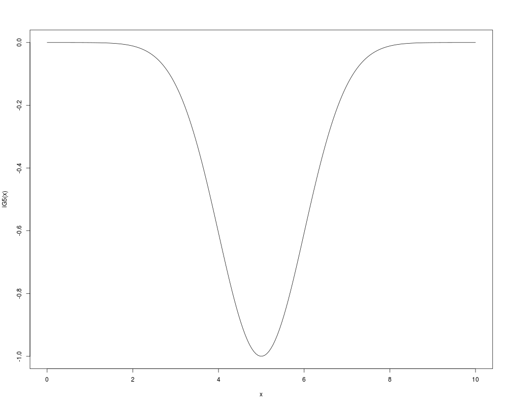
iG5 <- function(x) -exp(-(x-5)^2/2)
curve(iG5, 0, 10, 200)
o.dp  <- optimize (iG5, c(0, 10)) #->  5 of course
oM.gs <- optimizeR(iG5, 0, 10, method="Golden")
oM.Br <- optimizeR(iG5, 0, 10, method="Brent", trace=TRUE)
oM.gs$min ; oM.gs$iter
oM.Br$min ; oM.Br$iter
(doExtras <- Rmpfr:::doExtras())
if(doExtras) {## more accuracy {takes a few seconds}
 oM.gs <- optimizeR(iG5, 0, 10, method="Golden", tol = 1e-70)
 oM.Br <- optimizeR(iG5, 0, 10,                  tol = 1e-70)
}
rbind(Golden = c(err = as.numeric(oM.gs$min -5), iter = oM.gs$iter),
      Brent  = c(err = as.numeric(oM.Br$min -5), iter = oM.Br$iter))

## ==> Brent is orders of magnitude more efficient !

## Testing on the sine curve with 40 correct digits:
sol <- optimizeR(sin, 2, 6, tol = 1e-40)
str(sol)
sol <- optimizeR(sin, 2, 6, tol = 1e-50,
                 precFactor = 3.0, trace = TRUE)
pi.. <- 2*sol$min/3
print(pi.., digits=51)
stopifnot(all.equal(pi.., Const("pi", 256), tolerance = 10*1e-50))

if(doExtras) { # considerably more expensive

## a harder one:
f.sq <- function(x) sin(x-2)^4 + sqrt(pmax(0,(x-1)*(x-4)))*(x-2)^2
curve(f.sq, 0, 4.5, n=1000)
msq <- optimizeR(f.sq, 0, 5, tol = 1e-50, trace=5)
str(msq) # ok
stopifnot(abs(msq$minimum - 2) < 1e-49)

## find the other local minimum: -- non-smooth ==> Golden-section is used
msq2 <- optimizeR(f.sq, 3.5, 5, tol = 1e-50, trace=10)
stopifnot(abs(msq2$minimum - 4) < 1e-49)

## and a local maximum:
msq3 <- optimizeR(f.sq, 3, 4, maximum=TRUE, trace=2)
stopifnot(abs(msq3$maximum - 3.57) < 1e-2)

}#end {doExtras}


##----- "impossible" one to get precisely ------------------------

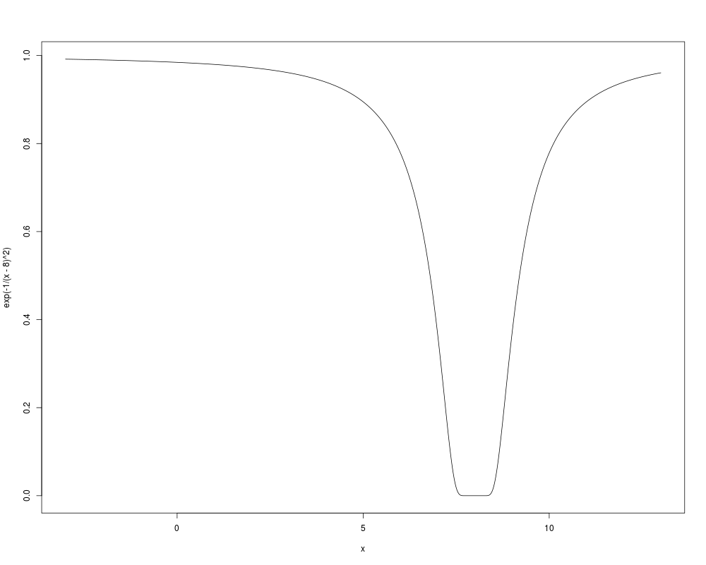
ff <- function(x) exp(-1/(x-8)^2)
curve(exp(-1/(x-8)^2), -3, 13, n=1001)
(opt. <- optimizeR(function(x) exp(-1/(x-8)^2), -3, 13, trace = 5))
## -> close to 8 {but not very close!}
ff(opt.$minimum) # gives 0
if(doExtras) {
 ## try harder ... in vain ..
 str(opt1 <- optimizeR(ff, -3,13, tol = 1e-60, precFactor = 4))
 print(opt1$minimum, digits=20)
 ## still just  7.99998038 or 8.000036655 {depending on method}
}

Results


R version 3.3.1 (2016-06-21) -- "Bug in Your Hair"
Copyright (C) 2016 The R Foundation for Statistical Computing
Platform: x86_64-pc-linux-gnu (64-bit)

R is free software and comes with ABSOLUTELY NO WARRANTY.
You are welcome to redistribute it under certain conditions.
Type 'license()' or 'licence()' for distribution details.

R is a collaborative project with many contributors.
Type 'contributors()' for more information and
'citation()' on how to cite R or R packages in publications.

Type 'demo()' for some demos, 'help()' for on-line help, or
'help.start()' for an HTML browser interface to help.
Type 'q()' to quit R.

> library(Rmpfr)
Loading required package: gmp

Attaching package: 'gmp'

The following objects are masked from 'package:base':

    %*%, apply, crossprod, matrix, tcrossprod

C code of R package 'Rmpfr': GMP using 64 bits per limb


Attaching package: 'Rmpfr'

The following objects are masked from 'package:stats':

    dbinom, dnorm, dpois, pnorm

The following objects are masked from 'package:base':

    cbind, pmax, pmin, rbind

> png(filename="/home/ddbj/snapshot/RGM3/R_CC/result/Rmpfr/optimizeR.Rd_%03d_medium.png", width=480, height=480)
> ### Name: optimizeR
> ### Title: High Precisione One-Dimensional Optimization
> ### Aliases: optimizeR
> ### Keywords: optimize
> 
> ### ** Examples
> 
> iG5 <- function(x) -exp(-(x-5)^2/2)
> curve(iG5, 0, 10, 200)
> o.dp  <- optimize (iG5, c(0, 10)) #->  5 of course
> oM.gs <- optimizeR(iG5, 0, 10, method="Golden")
> oM.Br <- optimizeR(iG5, 0, 10, method="Brent", trace=TRUE)
it.:   1, x = 3.8196601125       , delta(x) =         5 + Golden-Sect.
it.:   2, x = 6.1803398875       , delta(x) =    3.0902 + Golden-Sect.
it.:   3, x = 6.1803398875       , delta(x) =    1.9098 + Parabolic
it.:   4, x = 5                  , delta(x) =    1.1803 + Parabolic
it.:   5, x = 5                  , delta(x) =   0.59017 + Parabolic
> oM.gs$min ; oM.gs$iter
1 'mpfr' number of precision  132   bits 
[1] 5.0000000000000000000063125666903192147098
[1] 98
> oM.Br$min ; oM.Br$iter
1 'mpfr' number of precision  132   bits 
[1] 5.0000000000000000000000000000000000000029
[1] 6
> (doExtras <- Rmpfr:::doExtras())
[1] FALSE
> if(doExtras) {## more accuracy {takes a few seconds}
+  oM.gs <- optimizeR(iG5, 0, 10, method="Golden", tol = 1e-70)
+  oM.Br <- optimizeR(iG5, 0, 10,                  tol = 1e-70)
+ }
> rbind(Golden = c(err = as.numeric(oM.gs$min -5), iter = oM.gs$iter),
+       Brent  = c(err = as.numeric(oM.Br$min -5), iter = oM.Br$iter))
                err iter
Golden 6.312567e-21   98
Brent  2.938736e-39    6
> 
> ## ==> Brent is orders of magnitude more efficient !
> 
> ## Testing on the sine curve with 40 correct digits:
> sol <- optimizeR(sin, 2, 6, tol = 1e-40)
> str(sol)
List of 6
 $ minimum    :Class 'mpfr' [package "Rmpfr"] of length 1 and precision 265
 .. 4.71 
 $ objective  :Class 'mpfr' [package "Rmpfr"] of length 1 and precision 265
 .. -1 
 $ iter       : num 13
 $ convergence: logi TRUE
 $ estim.prec :Class 'mpfr' [package "Rmpfr"] of length 1 and precision 265
 .. 5.05e-40 
 $ method     : chr "Brent"
> sol <- optimizeR(sin, 2, 6, tol = 1e-50,
+                  precFactor = 3.0, trace = TRUE)
it.:   1, x = 3.527864045        , delta(x) =         2 + Golden-Sect.
it.:   2, x = 4.472135955        , delta(x) =    1.2361 + Golden-Sect.
it.:   3, x = 4.472135955        , delta(x) =   0.76393 + Parabolic
it.:   4, x = 4.70690584704      , delta(x) =    0.2918 + Parabolic
it.:   5, x = 4.7127462514       , delta(x) =   0.17441 + Parabolic
it.:   6, x = 4.71240160875      , delta(x) = 0.0029202 + Parabolic
it.:   7, x = 4.71238897995      , delta(x) = 0.0027479 + Parabolic
it.:   8, x = 4.71238898038      , delta(x) = 6.3144e-06 + Parabolic
it.:   9, x = 4.71238898038      , delta(x) = 6.3142e-06 + Parabolic
it.:  10, x = 4.71238898038      , delta(x) = 3.4767e-14 + Parabolic
it.:  11, x = 4.71238898038      , delta(x) = 3.4767e-14 + Parabolic
it.:  12, x = 4.71238898038      , delta(x) = 2.7062e-34 + Parabolic
it.:  13, x = 4.71238898038      , delta(x) = 2.9098e-49 + Parabolic
> pi.. <- 2*sol$min/3
> print(pi.., digits=51)
1 'mpfr' number of precision  498   bits 
[1] 3.14159265358979323846264338327950288419716939937511
> stopifnot(all.equal(pi.., Const("pi", 256), tolerance = 10*1e-50))
> 
> if(doExtras) { # considerably more expensive
+ 
+ ## a harder one:
+ f.sq <- function(x) sin(x-2)^4 + sqrt(pmax(0,(x-1)*(x-4)))*(x-2)^2
+ curve(f.sq, 0, 4.5, n=1000)
+ msq <- optimizeR(f.sq, 0, 5, tol = 1e-50, trace=5)
+ str(msq) # ok
+ stopifnot(abs(msq$minimum - 2) < 1e-49)
+ 
+ ## find the other local minimum: -- non-smooth ==> Golden-section is used
+ msq2 <- optimizeR(f.sq, 3.5, 5, tol = 1e-50, trace=10)
+ stopifnot(abs(msq2$minimum - 4) < 1e-49)
+ 
+ ## and a local maximum:
+ msq3 <- optimizeR(f.sq, 3, 4, maximum=TRUE, trace=2)
+ stopifnot(abs(msq3$maximum - 3.57) < 1e-2)
+ 
+ }#end {doExtras}
> 
> 
> ##----- "impossible" one to get precisely ------------------------
> 
> ff <- function(x) exp(-1/(x-8)^2)
> curve(exp(-1/(x-8)^2), -3, 13, n=1001)
> (opt. <- optimizeR(function(x) exp(-1/(x-8)^2), -3, 13, trace = 5))
it.:   5, x = 8.02127674502      , delta(x) =   0.85075 + Parabolic
it.:  10, x = 8.00702349232      , delta(x) =  0.014253 + Parabolic
it.:  15, x = 7.99989686597      , delta(x) =  0.003786 + Parabolic
it.:  20, x = 7.99999430031      , delta(x) = 1.3919e-05 + Golden-Sect.
it.:  25, x = 7.99998163622      , delta(x) = 1.0154e-06 + Golden-Sect.
it.:  30, x = 7.99998049429      , delta(x) = 9.1558e-08 + Golden-Sect.
it.:  35, x = 7.99998039133      , delta(x) = 8.2558e-09 + Golden-Sect.
it.:  40, x = 7.99998038204      , delta(x) = 7.4442e-10 + Golden-Sect.
it.:  45, x = 7.99998038121      , delta(x) = 6.7124e-11 + Golden-Sect.
it.:  50, x = 7.99998038113      , delta(x) = 6.0526e-12 + Golden-Sect.
it.:  55, x = 7.99998038112      , delta(x) = 5.4576e-13 + Golden-Sect.
it.:  60, x = 7.99998038112      , delta(x) = 4.9211e-14 + Golden-Sect.
it.:  65, x = 7.99998038112      , delta(x) = 4.4374e-15 + Golden-Sect.
it.:  70, x = 7.99998038112      , delta(x) = 4.0012e-16 + Golden-Sect.
it.:  75, x = 7.99998038112      , delta(x) = 3.6079e-17 + Golden-Sect.
it.:  80, x = 7.99998038112      , delta(x) = 3.2532e-18 + Golden-Sect.
it.:  85, x = 7.99998038112      , delta(x) = 2.9334e-19 + Golden-Sect.
$minimum
1 'mpfr' number of precision  132   bits 
[1] 7.9999803811226781163575244229367490051191

$objective
1 'mpfr' number of precision  132   bits 
[1] 0

$iter
[1] 87

$convergence
[1] TRUE

$estim.prec
1 'mpfr' number of precision  132   bits 
[1] 1.1204688214519642172286701602826826338935e-19

$method
[1] "Brent"

> ## -> close to 8 {but not very close!}
> ff(opt.$minimum) # gives 0
1 'mpfr' number of precision  132   bits 
[1] 0
> if(doExtras) {
+  ## try harder ... in vain ..
+  str(opt1 <- optimizeR(ff, -3,13, tol = 1e-60, precFactor = 4))
+  print(opt1$minimum, digits=20)
+  ## still just  7.99998038 or 8.000036655 {depending on method}
+ }
> 
> 
> 
> 
> 
> dev.off()
null device 
          1 
>