R Graphical Manual

Browse All

Last data update: 2014.03.03

R: Function to predict Rothermel's (1972) rate of spread [m/min]...

ros	R Documentation

Function to predict Rothermel's (1972) rate of spread [m/min] for surface headfires

Description

Include corrections to the orginal model by Frandsen (1973), Albini (1976), and Andrews et al. (2013).

Usage

ros (modeltype, w, s, delta, mx.dead, h, m, u, slope)

Arguments

`modeltype`	S(tatic), D(ynamic)
`w`	a vector or data frame of fuel load [t/ha] for fuel classes 1-hour, 10-hour, 100-hour, live herbs and live woody, respectively (5 values or columns; 0 if fuel class is absent).
`s`	a vector or data frame of surface-to-volume ratio [m2/m3] for fuel classes 1-hour, 10-hour, 100-hour, live herbs and live woody, respectively (5 values or columns; 0 if fuel class is absent).
`delta`	a value or vector of fuel bed depth [cm]
`mx.dead`	a value or vector of dead fuel moisture of extinction [percent]
`h`	a vector or data frame of heat content [kJ/kg] for fuel classes 1-hour, 10-hour, 100-hour, live herbs and live woody, respectively (5 values or columns; 0 if fuel class is absent).
`m`	a vector or data frame of percent moisture on a dry weight basis (percent) for fuel classes 1-hour, 10-hour, 100-hour, live herbs and live woody, respectively (5 values or columns; 0 if fuel class is absent).
`u`	a value or vector of midflame windspeed [km/h]
`slope`	a value or vector of site slope [percent]

Value

A list of values or vectors for the following variables: [1] Characteristic dead fuel moisture [percent], [2] Characteristic live fuel moisture [percent], [3] Live fuel moisture of extinction [percent], [4] Characteristic SAV [m2/m3] [5] Bulk density [kg/m3], [6] Packing ratio [dimensionless], [7] Relative packing ratio [dimensionless], [8] Dead fuel Reaction intensity [kW/m2], [9] Live fuel Reaction intensity [kW/m2], [10] Reaction intensity [kW/m2], [11] Wind factor [0-100], [12] Slope factor [0-1], [13] Heat source [kW/m2], [14] Heat sink [kJ/m3], [15] ROS [m/min].

Author(s)

Giorgio Vacchiano, Davide Ascoli (DISAFA, University of Torino, Italy)

References

Albini, F. A. (1976). Computer-based models of wildland fire behavior: A users' manual. Ogden, UT: US Department of Agriculture, Forest Service, Intermountain Forest and Range Experiment Station.

Andrews, P. L., Cruz, M. G., and Rothermel, R. C. (2013). Examination of the wind speed limit function in the Rothermel surface fire spread model. International Journal of Wildland Fire 22 (7): 959-969. http://dx.doi.org/10.1071/WF12122.

Frandsen, W. H. (1973). Using the effective heating number as a weighting factor in Rothermel's fire spread model. Ogden, UT: US Department of Agriculture, Forest Service, Intermountain Forest and Range Experiment Station.

Rothermel, R. C. (1972). A mathematical model for fire spread predictions in wildland fires. Research Paper INT-115. Ogden, UT: US Department of Agriculture, Forest Service, Intermountain Forest and Range Experiment Station.

Examples

# Example 1: Simulation using vectors of input values 

modeltype <- "D"
w <-c (2, 1, 0.5, 3, 8)
s <- c (5600, 358, 98, 6200, 8000)
delta <- 50
mx.dead <- 30
h <- c (18622, 18622, 18622, 19500, 20000)
m <- c (7, 8, 9, 40, 60)
u <- 5
slope <- 10

ros(modeltype, w, s, delta, mx.dead, h, m, u, slope)

# Example 2: variable wind input
# Only rate of spread is reported here (i.e., element [15] of ros ( ) output)

modeltype <- "D"
w <-c (2, 1, 0.5, 3, 8)
s <- c (5600, 358, 98, 6200, 8000)
delta <- 50
mx.dead <- 30
h <- c (18622, 18622, 18622, 19500, 20000)
m <- c (7, 8, 9, 40, 60)
slope <- 10

df <- data.frame ("windspeed" = seq (3, 15, 1), ROS=NA)

for (i in 1:nrow (df)) {
  df [i,2] <- 
  ros (modeltype, w, s, delta, mx.dead, h, m, u=df[i,1], slope) [15]
}
df

# Example 3: variable wind and slope input
# A two-entry table of rates of spread is created 

modeltype <- "D"
w <-c (2, 1, 0.5, 3, 8)
s <- c (5600, 358, 98, 6200, 8000)
delta <- 50
mx.dead <- 30
h <- c (18622, 18622, 18622, 19500, 20000)
m <- c (7, 8, 9, 40, 60)

u <- seq (3, 15, 1)
slope <- seq (0, 45, 15)

df <- matrix (rep (NA, length (u) * length (slope)), 
      length (u),
      length (slope)
      )
      
df <- data.frame (u, df)
colnames (df) <- c ("windspeed", 
  paste ("slope_", as.character (slope))
  )

for (i in 1:length (u)) {
  for (j in 1:length (slope)) {
    df [i, j+1] <- ros (
      modeltype, w, s, delta, mx.dead, h, m, u[i], slope[j])[15]
 }
}

df

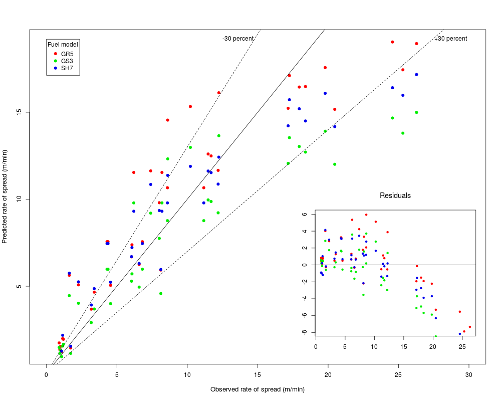
# Example 4: prediction and validation of rate of spread 
# using existing data from a field experiment

library (Rothermel)

# Observed variables
data (firexp) 
m <- firexp [, 18:22]
u <- firexp [, "u"]
slope <- firexp [, "slope"]
obs <- firexp [, "ros"]

# Predict ROS using Standard Fuel Models GR5, GS3 and SH7
data (SFM_metric)
a = list ( )
models = which (rownames (SFM_metric) == "GR5" |
      rownames (SFM_metric) == "GS3" |
      rownames (SFM_metric) == "SH7")
for (i in 1 : length (models) ) {
     modeltype <- SFM_metric [models [i], 1]
     w <- SFM_metric [models [i], 2:6]
     s <- SFM_metric [models [i], 7:11]
     delta <- SFM_metric [models [i], "Fuel_Bed_Depth"]
     mx.dead <- SFM_metric [models [i], "Mx_dead"]
     h <- SFM_metric [models [i], 14:18]
     a [i] <- ros (modeltype, w, s, delta, mx.dead, h,
        m, u, slope)[15]}
        
# Plot
plot (obs, a [[1]], xlab = "Observed rate of spread (m/min)",
         ylab = "Predicted rate of spread (m/min)",  col = "red",
         pch =19, xlim = c (0, 30), cex.lab = 1.1)
points (obs, a [[2]], pch = 19, col = "green2")
points (obs, a [[3]], pch = 19, col = "blue2")
abline (coef = c(0, 1))
abline (coef = c(0, 0.7),lty = 2); text (13.6, 19.2, "-30 percent")
abline (coef = c(0, 1.3),lty = 2); text (28.7, 19.2, "+30 percent")
legend (0, 19.2, c("GR5", "GS3", "SH7"), pch = 19,
        col = c("red", "green2", "blue2"), title = "Fuel model")

# Inset Residual plot (not run)
par (fig = c (.57, .98, .07, .55), new = TRUE)
plot (obs, a[[1]] - obs, xlab= "", ylab= "", col = "red",
       main= "Residuals", font.main = 1, pch=19, cex=.7)
points (obs, a [[2]] - obs, pch = 19, cex =.7, col = "green2")
points (obs, a [[3]] - obs, pch = 19, cex =.7, col = "blue2")
abline (h = 0)
par (fig = c (0, 1, 0, 1))

Results


R version 3.3.1 (2016-06-21) -- "Bug in Your Hair"
Copyright (C) 2016 The R Foundation for Statistical Computing
Platform: x86_64-pc-linux-gnu (64-bit)

R is free software and comes with ABSOLUTELY NO WARRANTY.
You are welcome to redistribute it under certain conditions.
Type 'license()' or 'licence()' for distribution details.

R is a collaborative project with many contributors.
Type 'contributors()' for more information and
'citation()' on how to cite R or R packages in publications.

Type 'demo()' for some demos, 'help()' for on-line help, or
'help.start()' for an HTML browser interface to help.
Type 'q()' to quit R.

> library(Rothermel)
Loading required package: GA
Loading required package: foreach
Loading required package: iterators
Package 'GA' version 3.0.2
Type 'citation("GA")' for citing this R package in publications.
Loading required package: ftsa
Loading required package: forecast
Loading required package: zoo

Attaching package: 'zoo'

The following objects are masked from 'package:base':

    as.Date, as.Date.numeric

Loading required package: timeDate
This is forecast 7.1 

Loading required package: rainbow
Loading required package: MASS
Loading required package: pcaPP
Loading required package: sde
Loading required package: stats4
Loading required package: fda
Loading required package: splines
Loading required package: Matrix

Attaching package: 'fda'

The following object is masked from 'package:forecast':

    fourier

The following object is masked from 'package:graphics':

    matplot

sde 2.0.15
Companion package to the book
'Simulation and Inference for Stochastic Differential Equations With R Examples'
Iacus, Springer NY, (2008)
To check the errata corrige of the book, type vignette("sde.errata")

Attaching package: 'ftsa'

The following objects are masked from 'package:stats':

    median, sd, var

> png(filename="/home/ddbj/snapshot/RGM3/R_CC/result/Rothermel/ros.Rd_%03d_medium.png", width=480, height=480)
> ### Name: ros
> ### Title: Function to predict Rothermel's (1972) rate of spread [m/min]
> ###   for surface headfires
> ### Aliases: ros
> ### Keywords: model
> 
> ### ** Examples
> 
> # Example 1: Simulation using vectors of input values 
> 
> modeltype <- "D"
> w <-c (2, 1, 0.5, 3, 8)
> s <- c (5600, 358, 98, 6200, 8000)
> delta <- 50
> mx.dead <- 30
> h <- c (18622, 18622, 18622, 19500, 20000)
> m <- c (7, 8, 9, 40, 60)
> u <- 5
> slope <- 10
> 
> ros(modeltype, w, s, delta, mx.dead, h, m, u, slope)
$`Characteristic dead fuel moisture [%]`
[1] 7.02

$`Characteristic live fuel moisture [%]`
[1] 59.37

$`Live fuel moisture of extinction [%]`
[1] 128.4

$`Characteristic SAV [m2/m3]`
[1] 7325.13

$`Bulk density [kg/m3]`
[1] 2.9

$`Packing ratio [dimensionless]`
[1] 0.0057

$`Relative packing ratio [dimensionless]`
[1] 0.93

$`Dead fuel Reaction intensity [kW/m2]`
[1] 553.34

$`Live fuel Reaction intensity [kW/m2]`
[1] 933.21

$`Reaction intensity [kW/m2]`
[1] 1486.55

$`Wind factor [0-100]`
[1] 6.75

$`Slope factor [0-1]`
[1] 0.25

$`Heat source [kW/m2]`
[1] 501.85

$`Heat sink [kJ/m3]`
[1] 4682.05

$`ROS [m/min]`
[1] 6.43

> 
> # Example 2: variable wind input
> # Only rate of spread is reported here (i.e., element [15] of ros ( ) output)
> 
> modeltype <- "D"
> w <-c (2, 1, 0.5, 3, 8)
> s <- c (5600, 358, 98, 6200, 8000)
> delta <- 50
> mx.dead <- 30
> h <- c (18622, 18622, 18622, 19500, 20000)
> m <- c (7, 8, 9, 40, 60)
> slope <- 10
> 
> df <- data.frame ("windspeed" = seq (3, 15, 1), ROS=NA)
> 
> for (i in 1:nrow (df)) {
+   df [i,2] <- 
+   ros (modeltype, w, s, delta, mx.dead, h, m, u=df[i,1], slope) [15]
+ }
> df
   windspeed   ROS
1          3  3.37
2          4  4.78
3          5  6.43
4          6  8.30
5          7 10.38
6          8 12.65
7          9 15.10
8         10 17.74
9         11 20.54
10        12 23.51
11        13 26.63
12        14 29.91
13        15 33.34
> 
> # Example 3: variable wind and slope input
> # A two-entry table of rates of spread is created 
> 
> modeltype <- "D"
> w <-c (2, 1, 0.5, 3, 8)
> s <- c (5600, 358, 98, 6200, 8000)
> delta <- 50
> mx.dead <- 30
> h <- c (18622, 18622, 18622, 19500, 20000)
> m <- c (7, 8, 9, 40, 60)
> 
> u <- seq (3, 15, 1)
> slope <- seq (0, 45, 15)
> 
> df <- matrix (rep (NA, length (u) * length (slope)), 
+       length (u),
+       length (slope)
+       )
>       
> df <- data.frame (u, df)
> colnames (df) <- c ("windspeed", 
+   paste ("slope_", as.character (slope))
+   )
> 
> for (i in 1:length (u)) {
+   for (j in 1:length (slope)) {
+     df [i, j+1] <- ros (
+       modeltype, w, s, delta, mx.dead, h, m, u[i], slope[j])[15]
+  }
+ }
> 
> df
   windspeed slope_ 0 slope_ 15 slope_ 30 slope_ 45
1          3     3.17      3.62      4.97      7.23
2          4     4.58      5.03      6.38      8.64
3          5     6.23      6.68      8.03     10.29
4          6     8.10      8.55      9.90     12.16
5          7    10.18     10.63     11.98     14.23
6          8    12.45     12.90     14.25     16.51
7          9    14.90     15.35     16.71     18.96
8         10    17.54     17.99     19.34     21.59
9         11    20.34     20.79     22.14     24.40
10        12    23.31     23.76     25.11     27.36
11        13    26.43     26.88     28.23     30.49
12        14    29.71     30.16     31.51     33.77
13        15    33.14     33.59     34.94     37.20
> 
> # Example 4: prediction and validation of rate of spread 
> # using existing data from a field experiment
> 
> library (Rothermel)
> 
> # Observed variables
> data (firexp) 
> m <- firexp [, 18:22]
> u <- firexp [, "u"]
> slope <- firexp [, "slope"]
> obs <- firexp [, "ros"]
> 
> # Predict ROS using Standard Fuel Models GR5, GS3 and SH7
> data (SFM_metric)
> a = list ( )
> models = which (rownames (SFM_metric) == "GR5" |
+       rownames (SFM_metric) == "GS3" |
+       rownames (SFM_metric) == "SH7")
> for (i in 1 : length (models) ) {
+      modeltype <- SFM_metric [models [i], 1]
+      w <- SFM_metric [models [i], 2:6]
+      s <- SFM_metric [models [i], 7:11]
+      delta <- SFM_metric [models [i], "Fuel_Bed_Depth"]
+      mx.dead <- SFM_metric [models [i], "Mx_dead"]
+      h <- SFM_metric [models [i], 14:18]
+      a [i] <- ros (modeltype, w, s, delta, mx.dead, h,
+         m, u, slope)[15]}
>         
> # Plot
> plot (obs, a [[1]], xlab = "Observed rate of spread (m/min)",
+          ylab = "Predicted rate of spread (m/min)",  col = "red",
+          pch =19, xlim = c (0, 30), cex.lab = 1.1)
> points (obs, a [[2]], pch = 19, col = "green2")
> points (obs, a [[3]], pch = 19, col = "blue2")
> abline (coef = c(0, 1))
> abline (coef = c(0, 0.7),lty = 2); text (13.6, 19.2, "-30 percent")
> abline (coef = c(0, 1.3),lty = 2); text (28.7, 19.2, "+30 percent")
> legend (0, 19.2, c("GR5", "GS3", "SH7"), pch = 19,
+         col = c("red", "green2", "blue2"), title = "Fuel model")
> 
> # Inset Residual plot (not run)
> par (fig = c (.57, .98, .07, .55), new = TRUE)
> plot (obs, a[[1]] - obs, xlab= "", ylab= "", col = "red",
+        main= "Residuals", font.main = 1, pch=19, cex=.7)
> points (obs, a [[2]] - obs, pch = 19, cex =.7, col = "green2")
> points (obs, a [[3]] - obs, pch = 19, cex =.7, col = "blue2")
> abline (h = 0)
> par (fig = c (0, 1, 0, 1))
> 
> 
> 
> 
> 
> 
> dev.off()
null device 
          1 
>