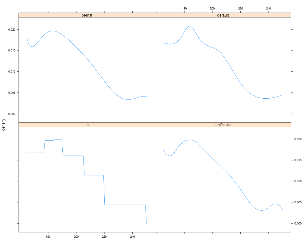
Semiparametric Elicitation of a bounded parameter.

Description

This package implements a novel method for fitting a bounded probability distribution to quantiles stated for example by an expert (see Bornkamp and Ickstadt (2009)). For this purpose B-splines are used, and the density is obtained by penalized least squares based on a Brier entropy penalty. The package provides methods for fitting the distribution as well as methods for evaluating the underlying density and cdf. In addition methods for plotting the distribution, drawing random numbers and calculating quantiles of the obtained distribution are provided.

Details

Author(s)

Bjoern Bornkamp

Maintainer: Bjoern Bornkamp <bornkamp@statistik.tu-dortmund.de>

References

Bornkamp, B. and Ickstadt, K. (2009). A Note on B-Splines for Semiparametric Elicitation. The American Statistician, 63, 373–377

O'Hagan A., Buck C. E., Daneshkhah, A., Eiser, R., Garthwaite, P., Jenkinson, D., Oakley, J. and Rakow, T. (2006), Uncertain Judgements: Eliciting Expert Probabilities, John Wiley and Sons Inc.

Garthwaite, P., Kadane, J. O'Hagan, A. (2005), Statistical Methods for Eliciting Probability Distributions, Journal of the American Statistical Association, 100, 680–701

Dierckx, P. (1993), Curve and Surface Fitting with Splines, Clarendon Press.

Examples

## example from O'Hagan et al. (2006)
x <- c(177.5, 183.75, 190, 205, 220)
y <- c(0.175, 0.33, 0.5, 0.75, 0.95)

default   <- SEL(x, y, Delta = 0.05, bounds = c(165, 250))
bernst    <- SEL(x, y, d = 10, N = 0, Delta = 0.05, bounds = c(165, 250))
unifknots <- SEL(x, y, d = 3, N = 5, Delta = 0.05, bounds = c(165, 250))
lin       <- SEL(x, y, d = 1, inknts = x, Delta = 0.05, bounds = c(165, 250))
comparePlot(default, bernst, unifknots, lin, type = "cdf")
comparePlot(default, bernst, unifknots, lin, type = "density")

## compare summaries
summary(default)
summary(bernst)
summary(unifknots)
summary(lin)

## sample from SEL object and evaluate density
xxx <- rvSEL(50000, bernst)
hist(xxx, breaks=100, freq=FALSE)
curve(predict(bernst, newdata=x), add=TRUE)

Results

R version 3.3.1 (2016-06-21) -- "Bug in Your Hair"
Copyright (C) 2016 The R Foundation for Statistical Computing
Platform: x86_64-pc-linux-gnu (64-bit)

R is free software and comes with ABSOLUTELY NO WARRANTY.
You are welcome to redistribute it under certain conditions.
Type 'license()' or 'licence()' for distribution details.

R is a collaborative project with many contributors.
Type 'contributors()' for more information and
'citation()' on how to cite R or R packages in publications.

Type 'demo()' for some demos, 'help()' for on-line help, or
'help.start()' for an HTML browser interface to help.
Type 'q()' to quit R.

> library(SEL)
Loading required package: splines
Loading required package: quadprog
Loading required package: lattice
> png(filename="/home/ddbj/snapshot/RGM3/R_CC/result/SEL/SEL-package.Rd_%03d_medium.png", width=480, height=480)
> ### Name: SEL-package
> ### Title: Semiparametric Elicitation of a bounded parameter.
> ### Aliases: SEL-package
> ### Keywords: package
> 
> ### ** Examples
> 
> ## example from O'Hagan et al. (2006)
> x <- c(177.5, 183.75, 190, 205, 220)
> y <- c(0.175, 0.33, 0.5, 0.75, 0.95)
> 
> default   <- SEL(x, y, Delta = 0.05, bounds = c(165, 250))
> bernst    <- SEL(x, y, d = 10, N = 0, Delta = 0.05, bounds = c(165, 250))
> unifknots <- SEL(x, y, d = 3, N = 5, Delta = 0.05, bounds = c(165, 250))
> lin       <- SEL(x, y, d = 1, inknts = x, Delta = 0.05, bounds = c(165, 250))
> comparePlot(default, bernst, unifknots, lin, type = "cdf")
> comparePlot(default, bernst, unifknots, lin, type = "density")
> 
> ## compare summaries
> summary(default)
    Min.  1st Qu.   Median  3rd Qu.     Max.     Mean     Var. 
165.0000 179.6175 192.4444 208.5933 250.0000 195.7178 419.5963 
> summary(bernst)
    Min.  1st Qu.   Median  3rd Qu.     Max.     Mean     Var. 
165.0000 179.4647 192.4660 208.5288 250.0000 195.6318 415.5795 
> summary(unifknots)
    Min.  1st Qu.   Median  3rd Qu.     Max.     Mean     Var. 
165.0000 179.5022 192.4060 208.7420 250.0000 195.6881 418.8084 
> summary(lin)
    Min.  1st Qu.   Median  3rd Qu.     Max.     Mean     Var. 
165.0000 179.5809 192.7284 209.6299 250.0000 196.1167 435.6236 
> 
> ## sample from SEL object and evaluate density
> xxx <- rvSEL(50000, bernst)
> hist(xxx, breaks=100, freq=FALSE)
> curve(predict(bernst, newdata=x), add=TRUE)
> 
> 
> 
> 
> 
> 
> 
> dev.off()
null device 
          1 
>