R Graphical Manual

Browse All

Last data update: 2014.03.03

R: PC-correlated SNPs in principal component analysis

snpgdsPCACorr

R Documentation

PC-correlated SNPs in principal component analysis

Description

To calculate the SNP correlations between eigenvactors and SNP genotypes

Usage

snpgdsPCACorr(pcaobj, gdsobj, snp.id=NULL, eig.which=NULL, num.thread=1L,
    verbose=TRUE)

Arguments

`pcaobj`	the `snpgdsPCAClass` object returned from the function snpgdsPCA
`gdsobj`	an object of class `SNPGDSFileClass`, a SNP GDS file
`snp.id`	a vector of snp id specifying selected SNPs; if NULL, all SNPs are used
`eig.which`	a vector of integers, to specify which eigenvectors to be used
`num.thread`	the number of (CPU) cores used; if `NA`, detect the number of cores automatically
`verbose`	if TRUE, show information

Value

Return a list:

`sample.id`	the sample ids used in the analysis
`snp.id`	the SNP ids used in the analysis
`snpcorr`	a matrix of correlation coefficients, "# of eigenvectors" x "# of SNPs"

Author(s)

Xiuwen Zheng

References

Patterson N, Price AL, Reich D (2006) Population structure and eigenanalysis. PLoS Genetics 2:e190.

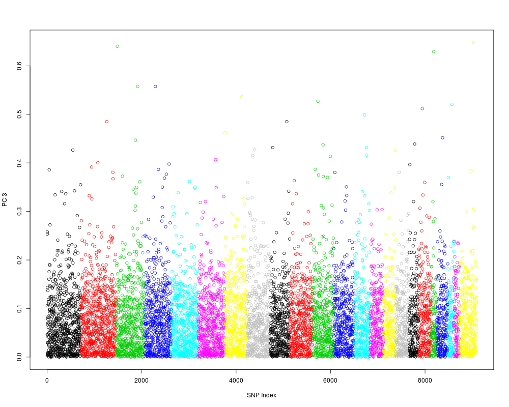
Examples

# open an example dataset (HapMap)
genofile <- snpgdsOpen(snpgdsExampleFileName())
# get chromosome index
chr <- read.gdsn(index.gdsn(genofile, "snp.chromosome"))

pca <- snpgdsPCA(genofile)
CORR <- snpgdsPCACorr(pca, genofile, eig.which=1:4)
plot(abs(CORR$snpcorr[3,]), xlab="SNP Index", ylab="PC 3", col=chr)

# close the file
snpgdsClose(genofile)

Results


R version 3.3.1 (2016-06-21) -- "Bug in Your Hair"
Copyright (C) 2016 The R Foundation for Statistical Computing
Platform: x86_64-pc-linux-gnu (64-bit)

R is free software and comes with ABSOLUTELY NO WARRANTY.
You are welcome to redistribute it under certain conditions.
Type 'license()' or 'licence()' for distribution details.

R is a collaborative project with many contributors.
Type 'contributors()' for more information and
'citation()' on how to cite R or R packages in publications.

Type 'demo()' for some demos, 'help()' for on-line help, or
'help.start()' for an HTML browser interface to help.
Type 'q()' to quit R.

> library(SNPRelate)
Loading required package: gdsfmt
SNPRelate -- supported by Streaming SIMD Extensions 2 (SSE2)
> png(filename="/home/ddbj/snapshot/RGM3/R_BC/result/SNPRelate/snpgdsPCACorr.Rd_%03d_medium.png", width=480, height=480)
> ### Name: snpgdsPCACorr
> ### Title: PC-correlated SNPs in principal component analysis
> ### Aliases: snpgdsPCACorr
> ### Keywords: PCA GDS GWAS
> 
> ### ** Examples
> 
> # open an example dataset (HapMap)
> genofile <- snpgdsOpen(snpgdsExampleFileName())
> # get chromosome index
> chr <- read.gdsn(index.gdsn(genofile, "snp.chromosome"))
> 
> pca <- snpgdsPCA(genofile)
Principal Component Analysis (PCA) on SNP genotypes:
Excluding 365 SNPs on non-autosomes
Excluding 1 SNP (monomorphic: TRUE, < MAF: NaN, or > missing rate: NaN)
Working space: 279 samples, 8722 SNPs
	using 1 (CPU) core
PCA:	the sum of all selected genotypes (0, 1 and 2) = 2446510
Wed Jul  6 05:34:47 2016    (internal increment: 1744)
 [>.................................................]  0%, ETC: NA     [==========>.......................................] 20%, ETC: 0s   [====================>.............................] 40%, ETC: 0s   [==============================>...................] 60%, ETC: 0s   [========================================>.........] 80%, ETC: 0s   [==================================================] 100%, ETC: 0s   [==================================================] 100%, completed  
Wed Jul  6 05:34:47 2016    Begin (eigenvalues and eigenvectors)
Wed Jul  6 05:34:47 2016    Done.
> CORR <- snpgdsPCACorr(pca, genofile, eig.which=1:4)
SNP correlation:
Working space: 279 samples, 9088 SNPs
	Using 1 (CPU) core.
	Using the top 32 eigenvectors.
SNP Correlation:	the sum of all selected genotypes (0, 1 and 2) = 2553065
Wed Jul  6 05:34:47 2016    (internal increment: 13976)
 [>.................................................]  0%, ETC: NA     [==================================================] 100%, completed  
Wed Jul  6 05:34:47 2016    Done.
> plot(abs(CORR$snpcorr[3,]), xlab="SNP Index", ylab="PC 3", col=chr)
> 
> # close the file
> snpgdsClose(genofile)
> 
> 
> 
> 
> 
> dev.off()
null device 
          1 
>