User friendly interface to class 'SampleSize'

Description

User friendly interface to class "SampleSize"

Usage

  sampleSize(PilotData,
    method = c("deconv", "congrad", "tikhonov", "ferreira"),
    control = list(from = -6, to = 6, resolution = 2^9))

Arguments

Details

The default method is 'deconv' which is an kernel deconvolution density estimator implementated using fft. The 'nncg' is a nonnegative conjugate gradient algorithm based on R's implementation see optim. 'tikonov' implements ridge-regression with optimal penalty selection using the L-curve approach. Higher order penalties are possible as well using a transformation to standard form (see Hansen).

The 'control' argument is a list that can supply any of the following components. Per method logical checks are performed.

• deconv:

  • method:'deconv', 'ferreira'

  • pi0Method:the pi0 estimation method one of 'Langaas', 'Storey', 'Ferreira', 'Userdefined'

  • pi0:if method = 'ferreira' grid pi0-value need to be suppled e.g. seq(0.1, 0.99, 0.01)

  • adjust:Default TRUE, adjust pi0 esitmate if density of effect size is somewhere negative.

  • a:Adjust pi0 better approach suggested by Efron. Symmetric range around zero of size 0.5.

  • bandwith:Default NULL uses 1/sqrt(log(length(statistics)))

  • kernel:Either 'fan', 'wand', 'sinc' kernels can be used.

  • from:Density of effect sizes should be estimated from = -6

  • to: to = 6

  • resolution:Density of effect sizes should be estimated on 2^9 points.

  • verbose:Default FALSE if TRUE additional information is printed to the console.

• congrad:

  • integration:'midpoint', 'trapezoidal', 'simpson'

  • scale:'pdfstat', 'cdfstat', 'cdfpval'

  • trim:0.01, 0.99

  • symmetric:TRUE

  • bin:'epdf', 'ecdf'

  • from:-6

  • to:6

  • resolution:500

  • verbose:Default FALSE if TRUE additional information is printed to the console.

• tikhonov:

  • integration:'midpoint', 'trapezoidal', 'simpson'

  • scale:'pdfstat', 'cdfstat', 'cdfpval'

  • trim:0.01, 0.99

  • symmetric:TRUE

  • bin:'epdf', 'ecdf'

  • from:-6

  • to:6

  • resolution:500

  • method:'lcurve', 'gcv', 'aic'

  • log:TRUE

  • penalty:0

  • lambda:10^seq(-10, 10, length=100)

  • verbose:Default FALSE if TRUE additional information is printed to the console.

• 'ferreira:'not yet implemeneted

Value

object of class SampleSize.

Author(s)

Maarten van Iterson

References

van Iterson, M., P. 't Hoen, P. Pedotti, G. Hooiveld, J. den Dunnen, G. van Ommen, J. Boer, and R. de Menezes (2009): 'Relative power and sample size analysis on gene expression profiling data,' BMC Genomics, 10, 439–449.

Ferreira, J. and A. Zwinderman (2006a): 'Approximate Power and Sample Size Calculations with the Benjamini-Hochberg Method,' The International Journal of Biostatistics, 2, 1.

Ferreira, J. and A. Zwinderman (2006b): 'Approximate Sample Size Calculations with Microarray Data: An Illustration,' Statistical Applications in Genetics and Molecular Biology, 5, 1.

Hansen, P. (2010): Discrete Inverse Problems: Insight and Algorithms, SIAM: Fun- damentals of algorithms series.

Langaas, M., B. Lindqvist, and E. Ferkingstad (2005): 'Estimating the proportion of true null hypotheses, with application to DNA microarray data,' Journal of the Royal Statistical Society Series B, 67, 555–572.

Storey, J. (2003): 'The positive false discovery rate: A bayesian interpretation and the q-value,' Annals of Statistics, 31, 2013–2035.

See Also

optim

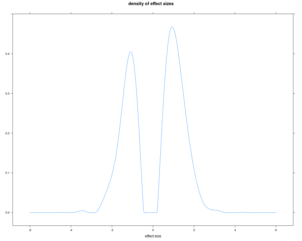
Examples

m <- 5000 ##number of genes
J <- 10 ##sample size per group
pi0 <- 0.8 ##proportion of non-differentially expressed genes
m0 <- as.integer(m*pi0)
mu <- rbitri(m - m0, a = log2(1.2), b = log2(4), m = log2(2)) #effect size distribution
data <- simdat(mu, m=m, pi0=pi0, J=J, noise=NULL)
library(genefilter)
stat <- rowttests(data, factor(rep(c(0, 1), each=J)), tstatOnly=TRUE)$statistic
pd <- pilotData(statistics=stat, samplesize=sqrt(J/2), distribution='norm')
ss <- sampleSize(pd, method='deconv')
plot(ss)

Results

R version 3.3.1 (2016-06-21) -- "Bug in Your Hair"
Copyright (C) 2016 The R Foundation for Statistical Computing
Platform: x86_64-pc-linux-gnu (64-bit)

R is free software and comes with ABSOLUTELY NO WARRANTY.
You are welcome to redistribute it under certain conditions.
Type 'license()' or 'licence()' for distribution details.

R is a collaborative project with many contributors.
Type 'contributors()' for more information and
'citation()' on how to cite R or R packages in publications.

Type 'demo()' for some demos, 'help()' for on-line help, or
'help.start()' for an HTML browser interface to help.
Type 'q()' to quit R.

> library(SSPA)
Loading required package: qvalue
Loading required package: lattice
Loading required package: limma
> png(filename="/home/ddbj/snapshot/RGM3/R_BC/result/SSPA/sampleSize.Rd_%03d_medium.png", width=480, height=480)
> ### Name: sampleSize
> ### Title: User friendly interface to class 'SampleSize'
> ### Aliases: sampleSize
> 
> ### ** Examples
> 
> m <- 5000 ##number of genes
> J <- 10 ##sample size per group
> pi0 <- 0.8 ##proportion of non-differentially expressed genes
> m0 <- as.integer(m*pi0)
> mu <- rbitri(m - m0, a = log2(1.2), b = log2(4), m = log2(2)) #effect size distribution
> data <- simdat(mu, m=m, pi0=pi0, J=J, noise=NULL)
> library(genefilter)
> stat <- rowttests(data, factor(rep(c(0, 1), each=J)), tstatOnly=TRUE)$statistic
> pd <- pilotData(statistics=stat, samplesize=sqrt(J/2), distribution='norm')
> ss <- sampleSize(pd, method='deconv')
> plot(ss)
> 
> 
> 
> 
> 
> dev.off()
null device 
          1 
>