Supported by Dr. Osamu Ogasawara and  . . |
|
Last data update: 2014.03.03 |
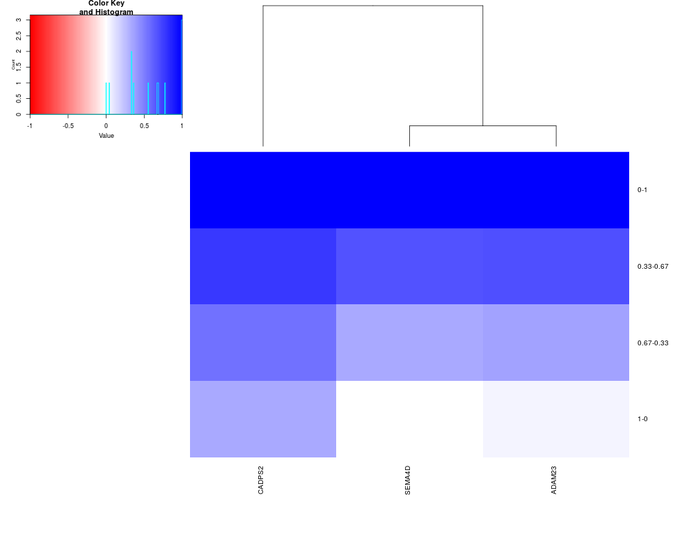
bioDistFeaturePlotDescriptionFunction that pltos the results from a bioDistFeature analysis UsagebioDistFeaturePlot(data) Arguments
ValueGenerates a heatmap plot Author(s)David Gomez-Cabrero Examples
data(STATegRa_S1)
data(STATegRa_S2)
require(Biobase)
# Truncate data for brevity
Block1 <- Block1[1:100,]
Block2 <- Block2[1:100,]
## Create ExpressionSets
mRNA.ds <- createOmicsExpressionSet(Data=Block1,pData=ed,pDataDescr=c("classname"))
miRNA.ds <- createOmicsExpressionSet(Data=Block2,pData=ed,pDataDescr=c("classname"))
## Create the bioMap
map.gene.miRNA<-bioMap(name = "Symbol-miRNA",
metadata = list(type_v1="Gene",type_v2="miRNA",
source_database="targetscan.Hs.eg.db",
data_extraction="July2014"),
map=mapdata)
# Create Gene-gene distance computed through miRNA data
bioDistmiRNA<-bioDist(referenceFeatures = rownames(Block1),
reference = "Var1",
mapping = map.gene.miRNA,
surrogateData = miRNA.ds, ### miRNA data
referenceData = mRNA.ds, ### mRNA data
maxitems=2,
selectionRule="sd",
expfac=NULL,
aggregation = "sum",
distance = "spearman",
noMappingDist = 0,
filtering = NULL,
name = "mRNAbymiRNA")
# Create Gene-gene distance through mRNA data
bioDistmRNA<-new("bioDistclass",
name = "mRNAbymRNA",
distance = cor(t(exprs(mRNA.ds)),method="spearman"),
map.name = "id",
map.metadata = list(),
params = list())
###### Generation of the list of Surrogated distances.
bioDistList<-list(bioDistmRNA,bioDistmiRNA)
sample.weights<-matrix(0,4,2)
sample.weights[,1]<-c(0,0.33,0.67,1)
sample.weights[,2]<-c(1,0.67,0.33,0)
###### Generation of the list of bioDistWclass objects.
bioDistWList<-bioDistW(referenceFeatures = rownames(Block1),
bioDistList = bioDistList,
weights=sample.weights)
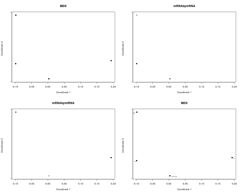
###### Plot of distances.
bioDistWPlot(referenceFeatures = rownames(Block1) ,
listDistW = bioDistWList,
method.cor="spearman")
###### Computing the matrix of features/distances associated.
fm<-bioDistFeature(Feature = rownames(Block1)[1] ,
listDistW = bioDistWList,
threshold.cor=0.7)
bioDistFeaturePlot(data=fm)
Results
R version 3.3.1 (2016-06-21) -- "Bug in Your Hair"
Copyright (C) 2016 The R Foundation for Statistical Computing
Platform: x86_64-pc-linux-gnu (64-bit)

R is free software and comes with ABSOLUTELY NO WARRANTY.
You are welcome to redistribute it under certain conditions.
Type 'license()' or 'licence()' for distribution details.

R is a collaborative project with many contributors.
Type 'contributors()' for more information and
'citation()' on how to cite R or R packages in publications.

Type 'demo()' for some demos, 'help()' for on-line help, or
'help.start()' for an HTML browser interface to help.
Type 'q()' to quit R.

> library(STATegRa)
Warning message:
replacing previous import 'Biobase::combine' by 'gridExtra::combine' when loading 'STATegRa'
> png(filename="/home/ddbj/snapshot/RGM3/R_BC/result/STATegRa/bioDistFeaturePlot.Rd_%03d_medium.png", width=480, height=480)
> ### Name: bioDistFeaturePlot
> ### Title: bioDistFeaturePlot
> ### Aliases: bioDistFeaturePlot
>
> ### ** Examples
>
> data(STATegRa_S1)
> data(STATegRa_S2)
> require(Biobase)
Loading required package: Biobase
Loading required package: BiocGenerics
Loading required package: parallel

Attaching package: 'BiocGenerics'

The following objects are masked from 'package:parallel':

    clusterApply, clusterApplyLB, clusterCall, clusterEvalQ,
    clusterExport, clusterMap, parApply, parCapply, parLapply,
    parLapplyLB, parRapply, parSapply, parSapplyLB

The following objects are masked from 'package:stats':

    IQR, mad, xtabs

The following objects are masked from 'package:base':

    Filter, Find, Map, Position, Reduce, anyDuplicated, append,
    as.data.frame, cbind, colnames, do.call, duplicated, eval, evalq,
    get, grep, grepl, intersect, is.unsorted, lapply, lengths, mapply,
    match, mget, order, paste, pmax, pmax.int, pmin, pmin.int, rank,
    rbind, rownames, sapply, setdiff, sort, table, tapply, union,
    unique, unsplit

Welcome to Bioconductor

    Vignettes contain introductory material; view with
    'browseVignettes()'. To cite Bioconductor, see
    'citation("Biobase")', and for packages 'citation("pkgname")'.

>
> # Truncate data for brevity
> Block1 <- Block1[1:100,]
> Block2 <- Block2[1:100,]
>
> ## Create ExpressionSets
> mRNA.ds <- createOmicsExpressionSet(Data=Block1,pData=ed,pDataDescr=c("classname"))
> miRNA.ds <- createOmicsExpressionSet(Data=Block2,pData=ed,pDataDescr=c("classname"))
>
> ## Create the bioMap
> map.gene.miRNA<-bioMap(name = "Symbol-miRNA",
+                        metadata =  list(type_v1="Gene",type_v2="miRNA",
+                                         source_database="targetscan.Hs.eg.db",
+                                         data_extraction="July2014"),
+                        map=mapdata)
>
> # Create Gene-gene distance computed through miRNA data
> bioDistmiRNA<-bioDist(referenceFeatures = rownames(Block1),
+                       reference = "Var1",
+                       mapping = map.gene.miRNA,
+                       surrogateData = miRNA.ds,  ### miRNA data
+                       referenceData = mRNA.ds,  ### mRNA data
+                       maxitems=2,
+                       selectionRule="sd",
+                       expfac=NULL,
+                       aggregation = "sum",
+                       distance = "spearman",
+                       noMappingDist = 0,
+                       filtering = NULL,
+                       name = "mRNAbymiRNA")
>
> # Create Gene-gene distance through mRNA data
> bioDistmRNA<-new("bioDistclass",
+                  name = "mRNAbymRNA",
+                  distance = cor(t(exprs(mRNA.ds)),method="spearman"),
+                  map.name = "id",
+                  map.metadata = list(),
+                  params = list())
>
> ###### Generation of the list of Surrogated distances.
>
> bioDistList<-list(bioDistmRNA,bioDistmiRNA)
> sample.weights<-matrix(0,4,2)
> sample.weights[,1]<-c(0,0.33,0.67,1)
> sample.weights[,2]<-c(1,0.67,0.33,0)
>
> ###### Generation of the list of bioDistWclass objects.
>
> bioDistWList<-bioDistW(referenceFeatures = rownames(Block1),
+                        bioDistList = bioDistList,
+                        weights=sample.weights)
>
> ###### Plot of distances.
> bioDistWPlot(referenceFeatures = rownames(Block1) ,
+              listDistW = bioDistWList,
+              method.cor="spearman")
Warning messages:
1: In cor.test.default(getDist(listDistW[[i]])[referenceFeatures, referenceFeatures],  :
  Cannot compute exact p-value with ties
2: In cor.test.default(getDist(listDistW[[i]])[referenceFeatures, referenceFeatures],  :
  Cannot compute exact p-value with ties
3: In cor.test.default(getDist(listDistW[[i]])[referenceFeatures, referenceFeatures],  :
  Cannot compute exact p-value with ties
4: In plot.window(...) :
  relative range of values =  10 * EPS, is small (axis 2)
5: In plot.window(...) :
  relative range of values =  10 * EPS, is small (axis 2)
6: In plot.window(...) :
  relative range of values =  10 * EPS, is small (axis 2)
7: In plot.window(...) :
  relative range of values =  10 * EPS, is small (axis 2)
>
> ###### Computing the matrix of features/distances associated.
>
> fm<-bioDistFeature(Feature = rownames(Block1)[1] ,
+                    listDistW = bioDistWList,
+                    threshold.cor=0.7)
> bioDistFeaturePlot(data=fm)
>
>
>
>
>
> dev.off()
null device
          1
>
|
Created & Maintained by Osamu Ogasawara (osamu.ogasawara@gmail.com) and 