Dirichlet Distribution

Description

Density function and random number generation for the Dirichlet distribution

Usage

rdirichlet(n, alpha)

Arguments

Value

The rdirichlet returns a matrix with n rows, each containing a single random number according to the supplied alpha vector or matrix.

Author(s)

Daniel Marcelino, dmarcelino@live.com

Examples

# 1) General usage:
rdirichlet(20, c(1,1,1) );
alphas <- cbind(1:10, 5, 10:1);
alphas;
rdirichlet(10, alphas );
alpha.0 <- sum( alphas );
test <- rdirichlet(10, alphas );
apply( test, 2, mean );
alphas / alpha.0;
apply( test, 2, var );
alphas * ( alpha.0 - alphas ) / ( alpha.0^2 * ( alpha.0 + 1 ) );

# 2) A practical example of usage:
# A Brazilian face-to-face poll by Datafolha conducted on Oct 03-04
# with 18,116 interviews asking for their vote preferences among the
# presidential candidates.

## First, draw a sample from the posterior
set.seed(1234);
n <- 18116;
poll <- c(40,24,22,5,5,4) / 100 * n; # The data
mcmc <- 100000;
sim <- rdirichlet(mcmc, alpha = poll + 1);

## Second, look at the margins of Aecio over Marina in the very last moment of the campaign:
margin <- sim[,2] - sim[,3];
mn <- mean(margin); # Bayes estimate
mn;
s <- sd(margin); # posterior standard deviation

qnts <- quantile(margin, probs = c(0.025, 0.975)); # 90% credible interval
qnts;
pr <- mean(margin > 0); # posterior probability of a positive margin
pr;

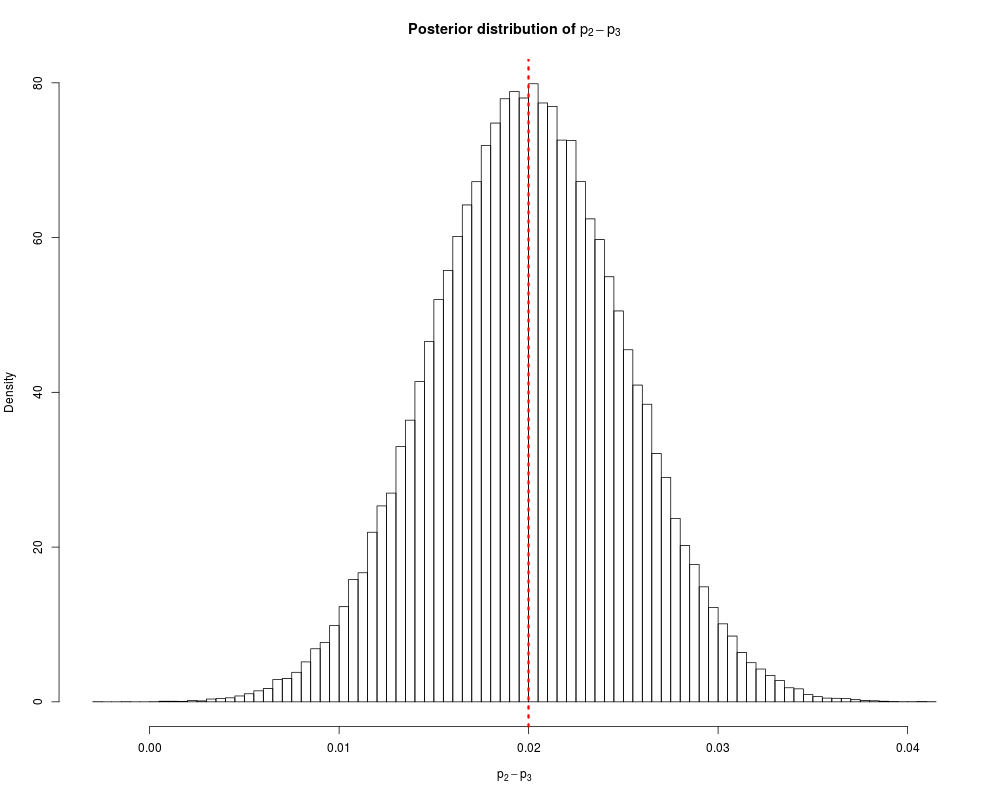
## Third, plot the posterior density
hist(margin, prob = TRUE, # posterior distribution
  breaks = "FD", xlab = expression(p[2] - p[3]),
  main = expression(paste(bold("Posterior distribution of "), p[2] - p[3])));
abline(v=mn, col='red', lwd=3, lty=3);

Results

R version 3.3.1 (2016-06-21) -- "Bug in Your Hair"
Copyright (C) 2016 The R Foundation for Statistical Computing
Platform: x86_64-pc-linux-gnu (64-bit)

R is free software and comes with ABSOLUTELY NO WARRANTY.
You are welcome to redistribute it under certain conditions.
Type 'license()' or 'licence()' for distribution details.

R is a collaborative project with many contributors.
Type 'contributors()' for more information and
'citation()' on how to cite R or R packages in publications.

Type 'demo()' for some demos, 'help()' for on-line help, or
'help.start()' for an HTML browser interface to help.
Type 'q()' to quit R.

> library(SciencesPo)
Loading required package: ggplot2
initializing ... done

> png(filename="/home/ddbj/snapshot/RGM3/R_CC/result/SciencesPo/rdirichlet.Rd_%03d_medium.png", width=480, height=480)
> ### Name: rdirichlet
> ### Title: Dirichlet Distribution
> ### Aliases: Dirichlet rdirichlet
> ### Keywords: Distributions
> 
> ### ** Examples
> 
> # 1) General usage:
> rdirichlet(20, c(1,1,1) );
             [,1]        [,2]        [,3]
 [1,] 0.391983852 0.068843511 0.539172637
 [2,] 0.646839431 0.195210432 0.157950137
 [3,] 0.014305348 0.832395924 0.153298727
 [4,] 0.521350308 0.359749440 0.118900252
 [5,] 0.563263490 0.049310117 0.387426393
 [6,] 0.003327916 0.401842460 0.594829624
 [7,] 0.783526221 0.116206369 0.100267410
 [8,] 0.693102051 0.294230742 0.012667207
 [9,] 0.382807400 0.506443431 0.110749169
[10,] 0.893229968 0.043618498 0.063151534
[11,] 0.094445936 0.787000462 0.118553602
[12,] 0.585686054 0.008558948 0.405754997
[13,] 0.733340992 0.079456937 0.187202072
[14,] 0.005813318 0.011039896 0.983146785
[15,] 0.006467625 0.975790023 0.017742352
[16,] 0.251262620 0.212643961 0.536093419
[17,] 0.189909608 0.477808464 0.332281928
[18,] 0.408441985 0.062612591 0.528945424
[19,] 0.136935884 0.249995408 0.613068708
[20,] 0.681390232 0.316528174 0.002081594
> alphas <- cbind(1:10, 5, 10:1);
> alphas;
      [,1] [,2] [,3]
 [1,]    1    5   10
 [2,]    2    5    9
 [3,]    3    5    8
 [4,]    4    5    7
 [5,]    5    5    6
 [6,]    6    5    5
 [7,]    7    5    4
 [8,]    8    5    3
 [9,]    9    5    2
[10,]   10    5    1
> rdirichlet(10, alphas );
            [,1]      [,2]       [,3]
 [1,] 0.15459091 0.3250877 0.52032143
 [2,] 0.08789328 0.3165045 0.59560221
 [3,] 0.14001528 0.2692944 0.59069032
 [4,] 0.29673442 0.1338062 0.56945941
 [5,] 0.30899708 0.2177496 0.47325330
 [6,] 0.32896735 0.3055050 0.36552770
 [7,] 0.46874047 0.2577410 0.27351854
 [8,] 0.37168783 0.1569000 0.47141220
 [9,] 0.51513945 0.3743110 0.11054955
[10,] 0.58521117 0.3991226 0.01566619
> alpha.0 <- sum( alphas );
> test <- rdirichlet(10, alphas );
> apply( test, 2, mean );
[1] 0.3652426 0.3442146 0.2905428
> alphas / alpha.0;
         [,1]    [,2]    [,3]
 [1,] 0.00625 0.03125 0.06250
 [2,] 0.01250 0.03125 0.05625
 [3,] 0.01875 0.03125 0.05000
 [4,] 0.02500 0.03125 0.04375
 [5,] 0.03125 0.03125 0.03750
 [6,] 0.03750 0.03125 0.03125
 [7,] 0.04375 0.03125 0.02500
 [8,] 0.05000 0.03125 0.01875
 [9,] 0.05625 0.03125 0.01250
[10,] 0.06250 0.03125 0.00625
> apply( test, 2, var );
[1] 0.069611132 0.009832517 0.046552147
> alphas * ( alpha.0 - alphas ) / ( alpha.0^2 * ( alpha.0 + 1 ) );
               [,1]         [,2]          [,3]
 [1,] 0.00003857725 0.0001880338 0.00036393634
 [2,] 0.00007666925 0.0001880338 0.00032972632
 [3,] 0.00011427601 0.0001880338 0.00029503106
 [4,] 0.00015139752 0.0001880338 0.00025985054
 [5,] 0.00018803377 0.0001880338 0.00022418478
 [6,] 0.00022418478 0.0001880338 0.00018803377
 [7,] 0.00025985054 0.0001880338 0.00015139752
 [8,] 0.00029503106 0.0001880338 0.00011427601
 [9,] 0.00032972632 0.0001880338 0.00007666925
[10,] 0.00036393634 0.0001880338 0.00003857725
> 
> # 2) A practical example of usage:
> # A Brazilian face-to-face poll by Datafolha conducted on Oct 03-04
> # with 18,116 interviews asking for their vote preferences among the
> # presidential candidates.
> 
> ## First, draw a sample from the posterior
> set.seed(1234);
> n <- 18116;
> poll <- c(40,24,22,5,5,4) / 100 * n; # The data
> mcmc <- 100000;
> sim <- rdirichlet(mcmc, alpha = poll + 1);
> 
> ## Second, look at the margins of Aecio over Marina in the very last moment of the campaign:
> margin <- sim[,2] - sim[,3];
> mn <- mean(margin); # Bayes estimate
> mn;
[1] 0.01999347
> s <- sd(margin); # posterior standard deviation
> 
> qnts <- quantile(margin, probs = c(0.025, 0.975)); # 90% credible interval
> qnts;
      2.5%      97.5% 
0.01018119 0.02990721 
> pr <- mean(margin > 0); # posterior probability of a positive margin
> pr;
[1] 0.99998
> 
> ## Third, plot the posterior density
> hist(margin, prob = TRUE, # posterior distribution
+   breaks = "FD", xlab = expression(p[2] - p[3]),
+   main = expression(paste(bold("Posterior distribution of "), p[2] - p[3])));
> abline(v=mn, col='red', lwd=3, lty=3);
> 
> 
> 
> 
> 
> dev.off()
null device 
          1 
>