Supported by Dr. Osamu Ogasawara and  . . |
|
Last data update: 2014.03.03 |
The ScottKnott Clustering Algoritm for Single ExperimentsDescriptionThese are methods for objects of class Usage
  ## Default S3 method:
SK(x,
   y=NULL,
   model,
   which,
   id.trim=3,
   error,
   sig.level=.05,
   dispersion=c('mm', 's', 'se'), ...)
  ## S3 method for class 'aov'
SK(x,
   which=NULL,
   id.trim=3,
   sig.level=.05,
   dispersion=c('mm', 's', 'se'), ...)
  ## S3 method for class 'aovlist'
SK(x,
   which,
   id.trim=3,
   error,
   sig.level=.05,
   dispersion=c('mm', 's', 'se'), ...)
Arguments
DetailsThe function The generic functions ValueThe function
Author(s)Enio Jelihovschi (eniojelihovs@gmail.com) ReferencesRamalho M.A.P., Ferreira D.F., Oliveira A.C. 2000. Experimenta<c3><a7><c3><a3>o em Gen<c3><a9>tica e Melhoramento de Plantas. Editora UFLA. Scott R.J., Knott M. 1974. A cluster analysis method for grouping mans in the analysis of variance. Biometrics, 30, 507-512. Examples
##
## Examples: Completely Randomized Design (CRD)
## More details: demo(package='ScottKnott')
##
## The parameters can be: vectors, design matrix and the response variable,
## data.frame or aov
data(CRD2)
## From: design matrix (dm) and response variable (y)
sk1 <- with(CRD2,
SK(x=dm,
y=y,
model='y ~ x',
which='x'))
summary(sk1)
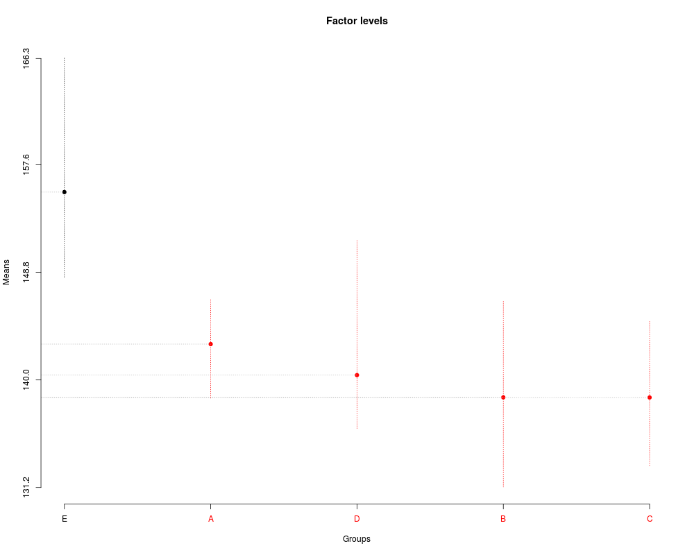
plot(sk1,
col=rainbow(max(sk1$groups)),
mm.lty=3,
id.las=2,
rl=FALSE,
title='factor levels')
## From: data.frame (dfm)
sk2 <- with(CRD2,
SK(x=dfm,
model='y ~ x',
which='x',
dispersion='s'))
summary(sk2)
plot(sk2,
col=rainbow(max(sk2$groups)),
id.las=2,
rl=FALSE)
## From: aov
av <- with(CRD2,
aov(y ~ x,
data=dfm))
summary(av)
sk3 <- with(CRD2,
SK(x=av,
which='x',
dispersion='se'))
summary(sk3)
plot(sk3,
col=rainbow(max(sk3$groups)),
rl=FALSE,
id.las=2,
title=NULL)
##
## Example: Randomized Complete Block Design (RCBD)
## More details: demo(package='ScottKnott')
##
## The parameters can be: design matrix and the response variable,
## data.frame or aov
data(RCBD)
## Design matrix (dm) and response variable (y)
sk1 <- with(RCBD,
SK(x=dm,
y=y,
model='y ~ blk + tra',
which='tra'))
summary(sk1)
plot(sk1)
## From: data.frame (dfm), which='tra'
sk2 <- with(RCBD,
SK(x=dfm,
model='y ~ blk + tra',
which='tra'))
summary(sk2)
plot(sk2,
mm.lty=3,
title='Factor levels')
##
## Example: Latin Squares Design (LSD)
## More details: demo(package='ScottKnott')
##
## The parameters can be: design matrix and the response variable,
## data.frame or aov
data(LSD)
## From: design matrix (dm) and response variable (y)
sk1 <- with(LSD,
SK(x=dm,
y=y,
model='y ~ rows + cols + tra',
which='tra'))
summary(sk1)
plot(sk1)
## From: data.frame
sk2 <- with(LSD,
SK(x=dfm,
model='y ~ rows + cols + tra',
which='tra'))
summary(sk2)
plot(sk2,
title='Factor levels')
## From: aov
av <- with(LSD,
aov(y ~ rows + cols + tra,
data=dfm))
summary(av)
sk3 <- SK(av,
which='tra')
summary(sk3)
plot(sk3,
title='Factor levels')
##
## Example: Factorial Experiment (FE)
## More details: demo(package='ScottKnott')
##
## The parameters can be: design matrix and the response variable,
## data.frame or aov
## Note: The factors are in uppercase and its levels in lowercase!
data(FE)
## From: design matrix (dm) and response variable (y)
## Main factor: N
sk1 <- with(FE,
SK(x=dm,
y=y,
model='y ~ blk + N*P*K',
which='N'))
summary(sk1)
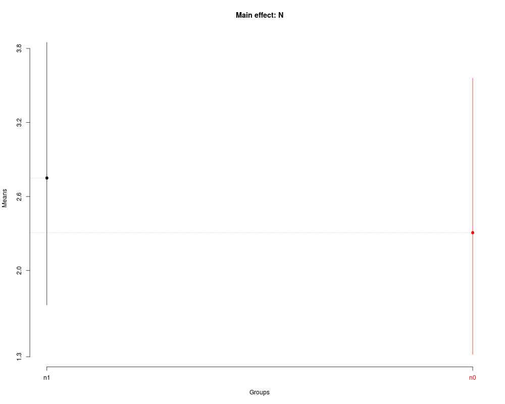
plot(sk1,
title='Main effect: N')
## Nested: p1/N
nsk1 <- with(FE,
SK.nest(x=dm,
y=y,
model='y ~ blk + N*P*K',
which='P:N',
fl1=1))
summary(nsk1)
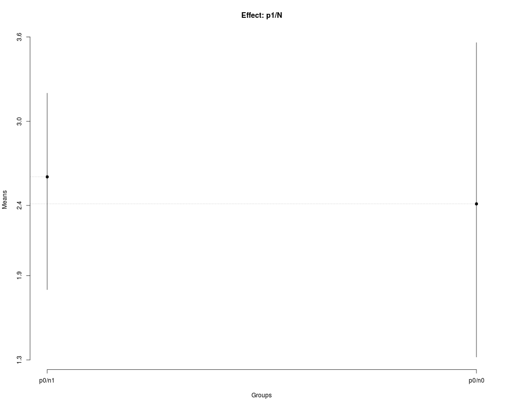
plot(nsk1,
title='Effect: p1/N')
Results
R version 3.3.1 (2016-06-21) -- "Bug in Your Hair"
Copyright (C) 2016 The R Foundation for Statistical Computing
Platform: x86_64-pc-linux-gnu (64-bit)
R is free software and comes with ABSOLUTELY NO WARRANTY.
You are welcome to redistribute it under certain conditions.
Type 'license()' or 'licence()' for distribution details.
R is a collaborative project with many contributors.
Type 'contributors()' for more information and
'citation()' on how to cite R or R packages in publications.
Type 'demo()' for some demos, 'help()' for on-line help, or
'help.start()' for an HTML browser interface to help.
Type 'q()' to quit R.
> library(ScottKnott)
> png(filename="/home/ddbj/snapshot/RGM3/R_CC/result/ScottKnott/SK.Rd_%03d_medium.png", width=480, height=480)
> ### Name: SK
> ### Title: The ScottKnott Clustering Algoritm for Single Experiments
> ### Aliases: SK SK.default SK.aov SK.aovlist
> ### Keywords: package htest univar tree design
>
> ### ** Examples
>
> ##
> ## Examples: Completely Randomized Design (CRD)
> ## More details: demo(package='ScottKnott')
> ##
>
> ## The parameters can be: vectors, design matrix and the response variable,
> ## data.frame or aov
> data(CRD2)
>
> ## From: design matrix (dm) and response variable (y)
> sk1 <- with(CRD2,
+ SK(x=dm,
+ y=y,
+ model='y ~ x',
+ which='x'))
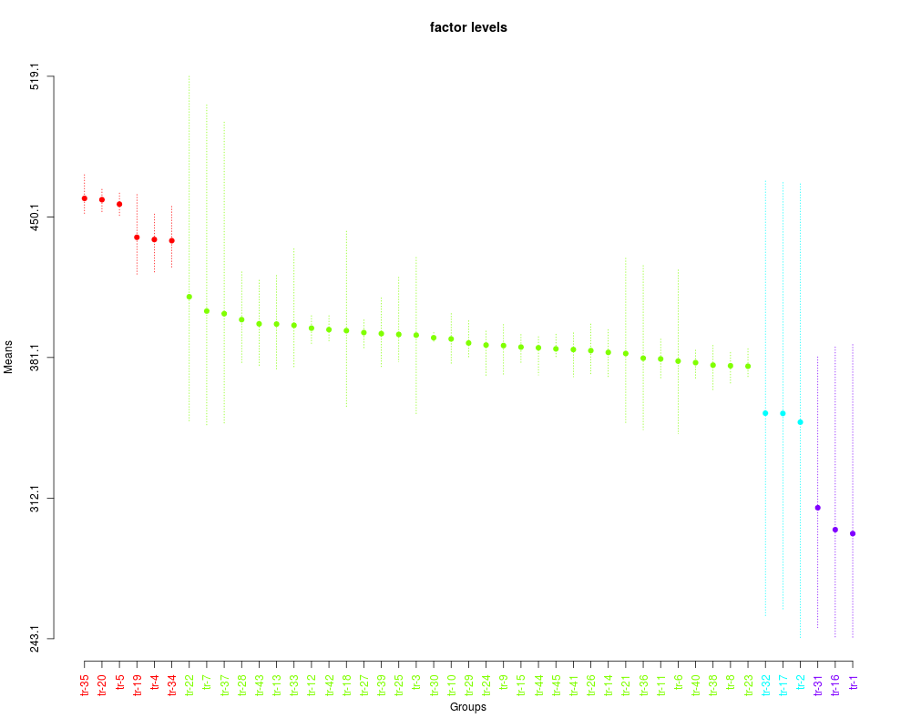
> summary(sk1)
Levels Means SK(5%)
tr-35 459.1650 a
tr-20 458.5300 a
tr-5 456.3500 a
tr-19 440.0750 a
tr-4 438.9850 a
tr-34 438.4225 a
tr-22 410.9100 b
tr-7 403.8800 b
tr-37 402.5925 b
tr-28 399.6675 b
tr-43 397.6000 b
tr-13 397.5025 b
tr-33 396.8950 b
tr-12 395.4875 b
tr-42 394.7650 b
tr-18 394.2600 b
tr-27 393.3200 b
tr-39 392.8200 b
tr-25 392.4100 b
tr-3 392.0725 b
tr-30 390.7950 b
tr-10 390.2025 b
tr-29 388.1975 b
tr-24 387.1950 b
tr-9 386.9500 b
tr-15 386.2050 b
tr-44 385.8675 b
tr-45 385.3325 b
tr-41 384.9825 b
tr-26 384.4675 b
tr-14 383.6075 b
tr-21 383.0625 b
tr-36 380.7450 b
tr-11 380.3875 b
tr-6 379.3175 b
tr-40 378.5675 b
tr-38 377.3475 b
tr-8 377.0425 b
tr-23 376.8125 b
tr-32 353.7575 c
tr-17 353.6525 c
tr-2 349.3500 c
tr-31 307.3700 d
tr-16 296.6125 d
tr-1 294.6800 d
> plot(sk1,
+ col=rainbow(max(sk1$groups)),
+ mm.lty=3,
+ id.las=2,
+ rl=FALSE,
+ title='factor levels')
>
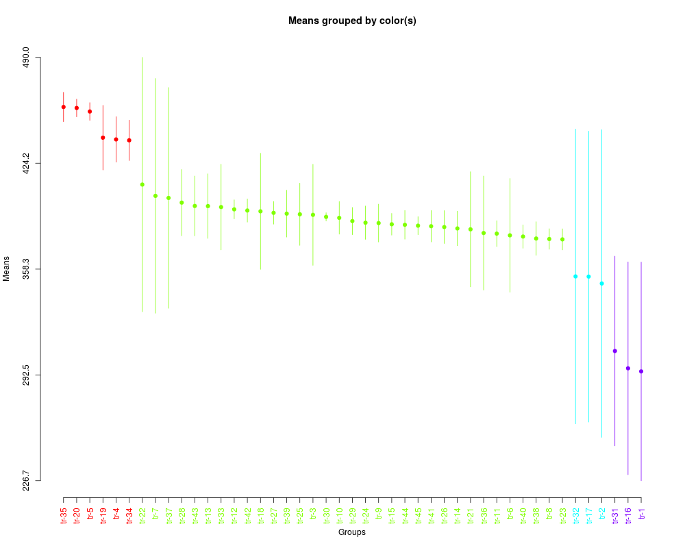
> ## From: data.frame (dfm)
> sk2 <- with(CRD2,
+ SK(x=dfm,
+ model='y ~ x',
+ which='x',
+ dispersion='s'))
> summary(sk2)
Levels Means SK(5%)
tr-35 459.1650 a
tr-20 458.5300 a
tr-5 456.3500 a
tr-19 440.0750 a
tr-4 438.9850 a
tr-34 438.4225 a
tr-22 410.9100 b
tr-7 403.8800 b
tr-37 402.5925 b
tr-28 399.6675 b
tr-43 397.6000 b
tr-13 397.5025 b
tr-33 396.8950 b
tr-12 395.4875 b
tr-42 394.7650 b
tr-18 394.2600 b
tr-27 393.3200 b
tr-39 392.8200 b
tr-25 392.4100 b
tr-3 392.0725 b
tr-30 390.7950 b
tr-10 390.2025 b
tr-29 388.1975 b
tr-24 387.1950 b
tr-9 386.9500 b
tr-15 386.2050 b
tr-44 385.8675 b
tr-45 385.3325 b
tr-41 384.9825 b
tr-26 384.4675 b
tr-14 383.6075 b
tr-21 383.0625 b
tr-36 380.7450 b
tr-11 380.3875 b
tr-6 379.3175 b
tr-40 378.5675 b
tr-38 377.3475 b
tr-8 377.0425 b
tr-23 376.8125 b
tr-32 353.7575 c
tr-17 353.6525 c
tr-2 349.3500 c
tr-31 307.3700 d
tr-16 296.6125 d
tr-1 294.6800 d
> plot(sk2,
+ col=rainbow(max(sk2$groups)),
+ id.las=2,
+ rl=FALSE)
>
> ## From: aov
> av <- with(CRD2,
+ aov(y ~ x,
+ data=dfm))
> summary(av)
Df Sum Sq Mean Sq F value Pr(>F)
x 44 209136 4753 3.273 7.69e-08 ***
Residuals 135 196045 1452
---
Signif. codes: 0 '***' 0.001 '**' 0.01 '*' 0.05 '.' 0.1 ' ' 1
>
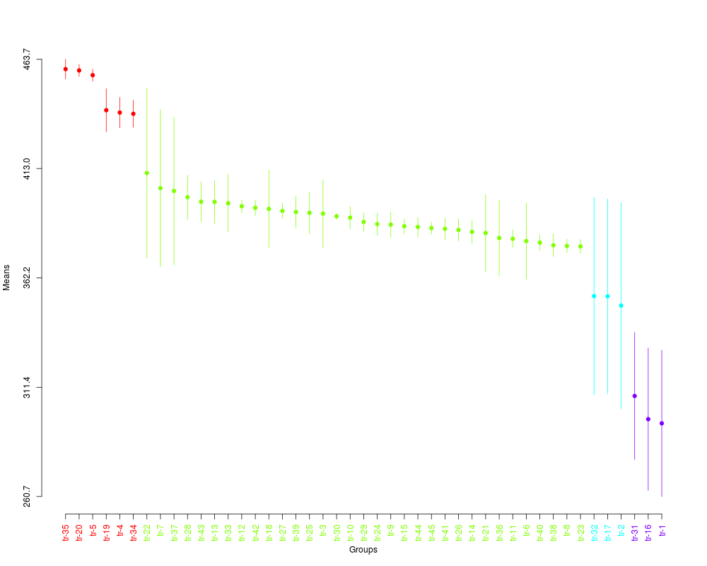
> sk3 <- with(CRD2,
+ SK(x=av,
+ which='x',
+ dispersion='se'))
> summary(sk3)
Levels Means SK(5%)
tr-35 459.1650 a
tr-20 458.5300 a
tr-5 456.3500 a
tr-19 440.0750 a
tr-4 438.9850 a
tr-34 438.4225 a
tr-22 410.9100 b
tr-7 403.8800 b
tr-37 402.5925 b
tr-28 399.6675 b
tr-43 397.6000 b
tr-13 397.5025 b
tr-33 396.8950 b
tr-12 395.4875 b
tr-42 394.7650 b
tr-18 394.2600 b
tr-27 393.3200 b
tr-39 392.8200 b
tr-25 392.4100 b
tr-3 392.0725 b
tr-30 390.7950 b
tr-10 390.2025 b
tr-29 388.1975 b
tr-24 387.1950 b
tr-9 386.9500 b
tr-15 386.2050 b
tr-44 385.8675 b
tr-45 385.3325 b
tr-41 384.9825 b
tr-26 384.4675 b
tr-14 383.6075 b
tr-21 383.0625 b
tr-36 380.7450 b
tr-11 380.3875 b
tr-6 379.3175 b
tr-40 378.5675 b
tr-38 377.3475 b
tr-8 377.0425 b
tr-23 376.8125 b
tr-32 353.7575 c
tr-17 353.6525 c
tr-2 349.3500 c
tr-31 307.3700 d
tr-16 296.6125 d
tr-1 294.6800 d
> plot(sk3,
+ col=rainbow(max(sk3$groups)),
+ rl=FALSE,
+ id.las=2,
+ title=NULL)
>
> ##
> ## Example: Randomized Complete Block Design (RCBD)
> ## More details: demo(package='ScottKnott')
> ##
>
> ## The parameters can be: design matrix and the response variable,
> ## data.frame or aov
>
> data(RCBD)
>
> ## Design matrix (dm) and response variable (y)
> sk1 <- with(RCBD,
+ SK(x=dm,
+ y=y,
+ model='y ~ blk + tra',
+ which='tra'))
> summary(sk1)
Levels Means SK(5%)
E 155.3700 a
A 142.9325 b
D 140.3950 b
B 138.5750 b
C 138.5650 b
> plot(sk1)
>
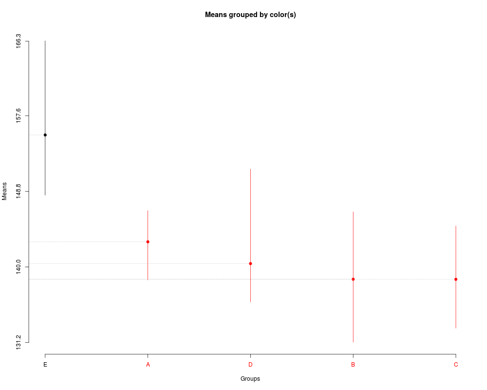
> ## From: data.frame (dfm), which='tra'
> sk2 <- with(RCBD,
+ SK(x=dfm,
+ model='y ~ blk + tra',
+ which='tra'))
> summary(sk2)
Levels Means SK(5%)
E 155.3700 a
A 142.9325 b
D 140.3950 b
B 138.5750 b
C 138.5650 b
> plot(sk2,
+ mm.lty=3,
+ title='Factor levels')
>
> ##
> ## Example: Latin Squares Design (LSD)
> ## More details: demo(package='ScottKnott')
> ##
>
> ## The parameters can be: design matrix and the response variable,
> ## data.frame or aov
>
> data(LSD)
>
> ## From: design matrix (dm) and response variable (y)
> sk1 <- with(LSD,
+ SK(x=dm,
+ y=y,
+ model='y ~ rows + cols + tra',
+ which='tra'))
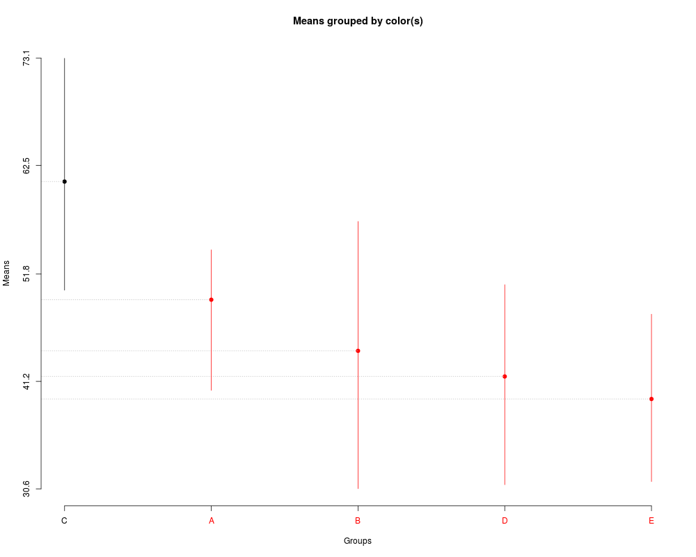
> summary(sk1)
Levels Means SK(5%)
C 60.910 a
A 49.258 b
B 44.216 b
D 41.686 b
E 39.464 b
> plot(sk1)
>
> ## From: data.frame
> sk2 <- with(LSD,
+ SK(x=dfm,
+ model='y ~ rows + cols + tra',
+ which='tra'))
> summary(sk2)
Levels Means SK(5%)
C 60.910 a
A 49.258 b
B 44.216 b
D 41.686 b
E 39.464 b
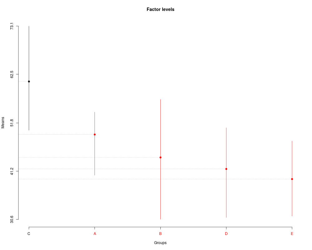
> plot(sk2,
+ title='Factor levels')
>
> ## From: aov
> av <- with(LSD,
+ aov(y ~ rows + cols + tra,
+ data=dfm))
> summary(av)
Df Sum Sq Mean Sq F value Pr(>F)
rows 4 398.8 99.7 4.193 0.023679 *
cols 4 589.9 147.5 6.201 0.006059 **
tra 4 1456.6 364.1 15.313 0.000116 ***
Residuals 12 285.4 23.8
---
Signif. codes: 0 '***' 0.001 '**' 0.01 '*' 0.05 '.' 0.1 ' ' 1
>
> sk3 <- SK(av,
+ which='tra')
> summary(sk3)
Levels Means SK(5%)
C 60.910 a
A 49.258 b
B 44.216 b
D 41.686 b
E 39.464 b
> plot(sk3,
+ title='Factor levels')
>
> ##
> ## Example: Factorial Experiment (FE)
> ## More details: demo(package='ScottKnott')
> ##
>
> ## The parameters can be: design matrix and the response variable,
> ## data.frame or aov
>
> ## Note: The factors are in uppercase and its levels in lowercase!
>
> data(FE)
> ## From: design matrix (dm) and response variable (y)
> ## Main factor: N
> sk1 <- with(FE,
+ SK(x=dm,
+ y=y,
+ model='y ~ blk + N*P*K',
+ which='N'))
> summary(sk1)
Levels Means SK(5%)
n1 2.750000 a
n0 2.306875 b
> plot(sk1,
+ title='Main effect: N')
>
> ## Nested: p1/N
> nsk1 <- with(FE,
+ SK.nest(x=dm,
+ y=y,
+ model='y ~ blk + N*P*K',
+ which='P:N',
+ fl1=1))
> summary(nsk1)
Nested: N/P
Levels Means SK(5%)
p0/n1 2.60375 a
p0/n0 2.41125 a
> plot(nsk1,
+ title='Effect: p1/N')
>
>
>
>
>
> dev.off()
null device
1
>
|