Supported by Dr. Osamu Ogasawara and  . . |
|
Last data update: 2014.03.03 |
The ScottKnott Clustering AlgorithmDescriptionThe Scott & Knott clustering algorithm is a very useful clustering algorithm widely used as a multiple comparison method in the Analysis of Variance context, as for example Gates and Bilbro (1978), Bony et al. (2001), Dilson et al. (2002) and Jyotsna et al. (2003). It was developed by Scott, A.J. and Knott, M. (Scott and Knott, 1974). All methods used up to that date as, for example, the t-test, Tukey, Duncan, Newman-Keuls procedures, have overlapping problems. By overlapping we mean the possibility of one or more treatments to be classified in more than one group, in fact, as the number of treatments reach a number of twenty or more, the number of overlappings could increse as reaching 5 or greater what makes almost impossible to the experimenter to really distinguish the real groups to which the means should belong. The Scott & Knott method does not have this problem, what is often cited as a very good quality of this procedure. The Scott & Knott method make use of a clever algorithm of cluster analysis, where, starting from the the whole group of observed mean effects, it divides, and keep dividing the sub-groups in such a way that the intersection of any two groups formed in that manner is empty. Using their own words 'we study the consequences of using a well-known method of cluster analysis to partition the sample treatment means in a balanced design and show how a corresponding likelihood ratio test gives a method of judging the significance of difference among groups abtained'. Many studies, using the method of Monte Carlo, suggest that the Scott Knott
method performs very well compared to other methods due to fact that it has
high power and type I error rate almost always in accordance with the nominal
levels. The ScottKnott package performs this algorithm starting either from
In a few words, the test of Scott & Knott is a clustering algorithm used as an one of the alternatives where multiple comparizon procedures are applied with a very important and almost unique characteristic: it does not present overlapping in the results. Author(s)Enio Jelihovschi (eniojelihovs@gmail.com) ReferencesBony S., Pichon N., Ravel C., Durix A., Balfourier F., Guillaumin J.J. 2001. The Relationship be-tween Mycotoxin Synthesis and Isolate Morphology in Fungal Endophytes of Lolium perenne. New Phytologist, 1521, 125-137. Borges L.C., FERREIRA D.F. 2003. Poder e taxas de erro tipo I dos testes Scott-Knott, Tukey e Student-Newman-Keuls sob distribuicoes normal e nao normais dos residuos. Power and type I errors rate of Scott-Knott, Tukey and Student-Newman-Keuls tests under normal and no-normal distributions of the residues. Rev. Mat. Estat., Sao Paulo, 211: 67-83. Calinski T., Corsten L.C.A. 1985. Clustering Means in ANOVA by Simultaneous Testing. Bio-metrics, 411, 39-48. Da Silva E.C, Ferreira D.F, Bearzoti E. 1999. Evaluation of power and type I error rates of Scott-Knotts test by the method of Monte Carlo. Cienc. agrotec., Lavras, 23, 687-696. Dilson A.B, David S.D., Kazimierz J., William W.K. 2002. Half-sib progeny evaluation and selection of potatoes resistant to the US8 genotype of Phytophthora infestans from crosses between resistant and susceptible parents. Euphytica, 125, 129-138. Gates C.E., Bilbro J.D. 1978. Illustration of a Cluster Analysis Method for Mean Separation. Agron J, 70, 462-465. Wilkinson, G.N, Rogers, C.E. 1973. Journal of the Royal Statistical Society. Series C (Applied Statistics), Vol. 22, No. 3, pp. 392-399. Jyotsna S., Zettler L.W., van Sambeek J.W., Ellersieck M.R., Starbuck C.J. 2003. Symbiotic Seed Germination and Mycorrhizae of Federally Threatened Platanthera PraeclaraOrchidaceae. American Midland Naturalist, 1491, 104-120. Ramalho M.A.P., Ferreira DF, Oliveira AC 2000. Experimenta<c3><a7><c3><a3>o em Gen<c3><a9>tica e Melhoramento de Plantas. Editora UFLA. Scott R.J., Knott M. 1974. A cluster analysis method for grouping mans in the analysis of variance. Biometrics, 30, 507-512. Examples
##
## Examples: Completely Randomized Design (CRD)
## More details: demo(package='ScottKnott')
##
## The parameters can be: vectors, design matrix and the response variable,
## data.frame or aov
data(CRD2)
## From: design matrix (dm) and response variable (y)
sk1 <- with(CRD2,
SK(x=dm,
y=y,
model='y ~ x',
which='x'))
summary(sk1)
plot(sk1,
col=rainbow(max(sk1$groups)),
mm.lty=3,
id.las=2,
rl=FALSE,
title='Factor levels')
## From: data.frame (dfm)
sk2 <- with(CRD2,
SK(x=dfm,
model='y ~ x',
which='x',
dispersion='se'))
summary(sk2)
plot(sk2,
col=rainbow(max(sk2$groups)),
id.las=2,
rl=FALSE)
## From: aov
av <- with(CRD2,
aov(y ~ x,
data=dfm))
summary(av)
sk3 <- SK(x=av,
which='x')
summary(sk3)
plot(sk3,
col=rainbow(max(sk3$groups)),
rl=FALSE,
id.las=2,
title=NULL)
##
## Example: Randomized Complete Block Design (RCBD)
## More details: demo(package='ScottKnott')
##
## The parameters can be: design matrix and the response variable,
## data.frame or aov
data(RCBD)
## Design matrix (dm) and response variable (y)
sk1 <- with(RCBD,
SK(x=dm,
y=y,
model='y ~ blk + tra',
which='tra'))
summary(sk1)
plot(sk1)
## From: data.frame (dfm), which='tra'
sk2 <- with(RCBD,
SK(x=dfm,
model='y ~ blk + tra',
which='tra'))
summary(sk2)
plot(sk2,
mm.lty=3,
title='Factor levels')
##
## Example: Latin Squares Design (LSD)
## More details: demo(package='ScottKnott')
##
## The parameters can be: design matrix and the response variable,
## data.frame or aov
data(LSD)
## From: design matrix (dm) and response variable (y)
sk1 <- with(LSD,
SK(x=dm,
y=y,
model='y ~ rows + cols + tra',
which='tra'))
summary(sk1)
plot(sk1)
## From: data.frame
sk2 <- with(LSD,
SK(x=dfm,
model='y ~ rows + cols + tra',
which='tra'))
summary(sk2)
plot(sk2,
title='Factor levels')
## From: aov
av <- with(LSD,
aov(y ~ rows + cols + tra,
data=dfm))
summary(av)
sk3 <- SK(av,
which='tra')
summary(sk3)
plot(sk3,
title='Factor levels')
##
## Example: Factorial Experiment (FE)
## More details: demo(package='ScottKnott')
##
## The parameters can be: design matrix and the response variable,
## data.frame or aov
## Note: The factors are in uppercase and its levels in lowercase!
data(FE)
## From: design matrix (dm) and response variable (y)
## Main factor: N
sk1 <- with(FE,
SK(x=dm,
y=y,
model='y ~ blk + N*P*K',
which='N'))
summary(sk1)
plot(sk1,
title='Main effect: N')
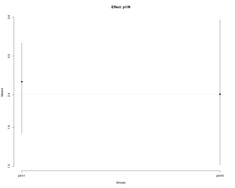
## Nested: p1/N
## Studing N inside of level one of P
nsk1 <- with(FE,
SK.nest(x=dm,
y=y,
model='y ~ blk + N*P*K',
which='P:N',
fl1=1))
summary(nsk1)
plot(nsk1,
title='Effect: p1/N')
## Nested: k1/P
nsk2 <- with(FE,
SK.nest(x=dm,
y=y,
model='y ~ blk + N*P*K',
which='K:P',
fl1=1))
summary(nsk2)
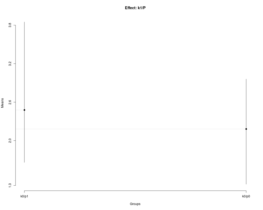
plot(nsk2,
title='Effect: k1/P')
## Nested: k2/p2/N
nsk3 <- with(FE,
SK.nest(x=dm,
y=y,
model='y ~ blk + N*P*K',
which='K:P:N',
fl1=2,
fl2=2))
summary(nsk3)
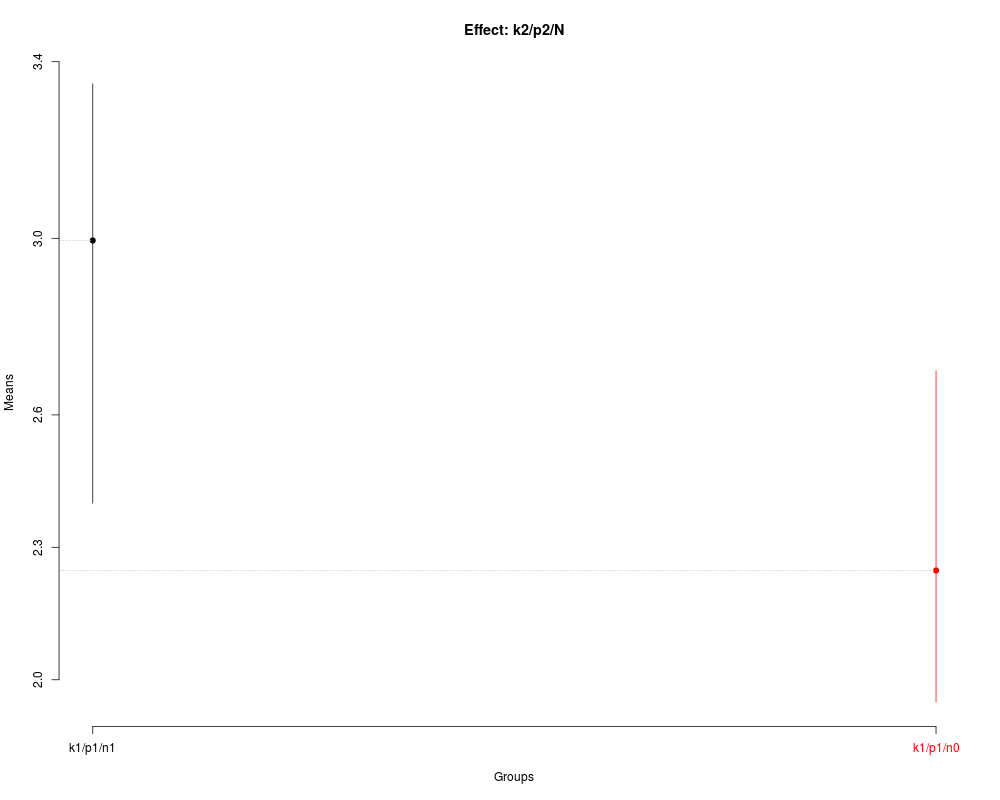
plot(nsk3,
title='Effect: k2/p2/N')
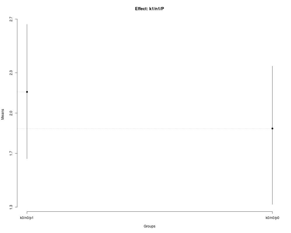
## Nested: k1/n1/P
## Studing P inside of level one of K and level one of N
nsk4 <- with(FE,
SK.nest(x=dm,
y=y,
model='y ~ blk + N*P*K',
which='K:N:P',
fl1=1,
fl2=1))
summary(nsk4)
plot(nsk4,
title='Effect: k1/n1/P')
## Nested: p1/n1/K
nsk5 <- with(FE,
SK.nest(x=dm,
y=y,
model='y ~ blk + N*P*K',
which='P:N:K',
fl1=1,
fl2=1))
summary(nsk5)
plot(nsk5, title='Effect: p1/n1/K')
##
## Example: Split-plot Experiment (SPE)
## More details: demo(package='ScottKnott')
##
## Note: The factors are in uppercase and its levels in lowercase!
data(SPE)
## The parameters can be: design matrix and the response variable,
## data.frame or aov
## From: design matrix (dm) and response variable (y)
## Main factor: P
sk1 <- with(SPE,
SK(x=dm,
y=y,
model='y ~ blk + P*SP + Error(blk/P)',
which='P',
error='blk:P'))
summary(sk1)
plot(sk1)
## Main factor: SP
sk2 <- with(SPE,
SK(x=dm,
y=y,
model='y ~ blk + P*SP + Error(blk/P)',
which='SP',
error='Within'))
summary(sk2)
plot(sk2,
xlab='Groups',
ylab='Main effect: sp',
title='Main effect: SP')
## Nested: p1/SP
skn1 <- with(SPE,
SK.nest(x=dm,
y=y,
model='y ~ blk + P*SP + Error(blk/P)',
which='P:SP',
error='Within',
fl1=1 ))
summary(skn1)
plot(skn1,
title='Effect: p1/SP')
##
## Example: Split-split-plot Experiment (SSPE)
## More details: demo(package='ScottKnott')
##
## Note: The factors are in uppercase and its levels in lowercase!
data(SSPE)
## From: design matrix (dm) and response variable (y)
## Main factor: P
sk1 <- with(SSPE,
SK(dm,
y,
model='y ~ blk + P*SP*SSP + Error(blk/P/SP)',
which='P',
error='blk:P'))
summary(sk1)
# Main factor: SP
sk2 <- with(SSPE,
SK(dm,
y,
model='y ~ blk + P*SP*SSP + Error(blk/P/SP)',
which='SP',
error='blk:P:SP'))
summary(sk2)
# Main factor: SSP
sk3 <- with(SSPE,
SK(dm,
y,
model='y ~ blk + P*SP*SSP + Error(blk/P/SP)',
which='SSP',
error='Within'))
summary(sk3)
## Nested: p1/SP
skn1 <- with(SSPE,
SK.nest(dm,
y,
model='y ~ blk + P*SP*SSP + Error(blk/P/SP)',
which='P:SP',
error='blk:P:SP',
fl1=1))
summary(skn1)
## From: aovlist
av <- with(SSPE,
aov(y ~ blk + P*SP*SSP + Error(blk/P/SP),
data=dfm))
summary(av)
## Nested: p/sp/SSP (at various levels of sp and p)
skn6 <- SK.nest(av,
which='P:SP:SSP',
error='Within',
fl1=1,
fl2=1)
summary(skn6)
skn7 <- SK.nest(av,
which='P:SP:SSP',
error='Within',
fl1=2,
fl2=1)
summary(skn7)
Results
R version 3.3.1 (2016-06-21) -- "Bug in Your Hair"
Copyright (C) 2016 The R Foundation for Statistical Computing
Platform: x86_64-pc-linux-gnu (64-bit)
R is free software and comes with ABSOLUTELY NO WARRANTY.
You are welcome to redistribute it under certain conditions.
Type 'license()' or 'licence()' for distribution details.
R is a collaborative project with many contributors.
Type 'contributors()' for more information and
'citation()' on how to cite R or R packages in publications.
Type 'demo()' for some demos, 'help()' for on-line help, or
'help.start()' for an HTML browser interface to help.
Type 'q()' to quit R.
> library(ScottKnott)
> png(filename="/home/ddbj/snapshot/RGM3/R_CC/result/ScottKnott/ScottKnott-package.Rd_%03d_medium.png", width=480, height=480)
> ### Name: ScottKnott-package
> ### Title: The ScottKnott Clustering Algorithm
> ### Aliases: ScottKnott-package ScottKnott
> ### Keywords: package htest univar tree design
>
> ### ** Examples
>
> ##
> ## Examples: Completely Randomized Design (CRD)
> ## More details: demo(package='ScottKnott')
> ##
>
> ## The parameters can be: vectors, design matrix and the response variable,
> ## data.frame or aov
> data(CRD2)
>
> ## From: design matrix (dm) and response variable (y)
> sk1 <- with(CRD2,
+ SK(x=dm,
+ y=y,
+ model='y ~ x',
+ which='x'))
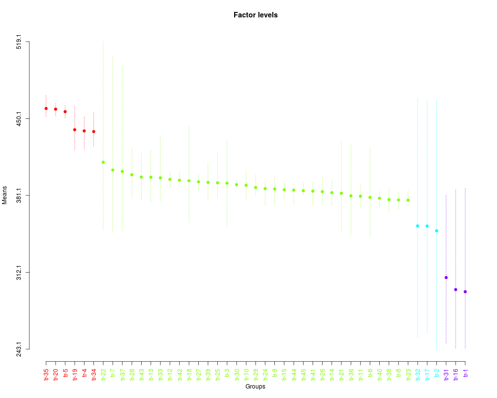
> summary(sk1)
Levels Means SK(5%)
tr-35 459.1650 a
tr-20 458.5300 a
tr-5 456.3500 a
tr-19 440.0750 a
tr-4 438.9850 a
tr-34 438.4225 a
tr-22 410.9100 b
tr-7 403.8800 b
tr-37 402.5925 b
tr-28 399.6675 b
tr-43 397.6000 b
tr-13 397.5025 b
tr-33 396.8950 b
tr-12 395.4875 b
tr-42 394.7650 b
tr-18 394.2600 b
tr-27 393.3200 b
tr-39 392.8200 b
tr-25 392.4100 b
tr-3 392.0725 b
tr-30 390.7950 b
tr-10 390.2025 b
tr-29 388.1975 b
tr-24 387.1950 b
tr-9 386.9500 b
tr-15 386.2050 b
tr-44 385.8675 b
tr-45 385.3325 b
tr-41 384.9825 b
tr-26 384.4675 b
tr-14 383.6075 b
tr-21 383.0625 b
tr-36 380.7450 b
tr-11 380.3875 b
tr-6 379.3175 b
tr-40 378.5675 b
tr-38 377.3475 b
tr-8 377.0425 b
tr-23 376.8125 b
tr-32 353.7575 c
tr-17 353.6525 c
tr-2 349.3500 c
tr-31 307.3700 d
tr-16 296.6125 d
tr-1 294.6800 d
> plot(sk1,
+ col=rainbow(max(sk1$groups)),
+ mm.lty=3,
+ id.las=2,
+ rl=FALSE,
+ title='Factor levels')
>
> ## From: data.frame (dfm)
> sk2 <- with(CRD2,
+ SK(x=dfm,
+ model='y ~ x',
+ which='x',
+ dispersion='se'))
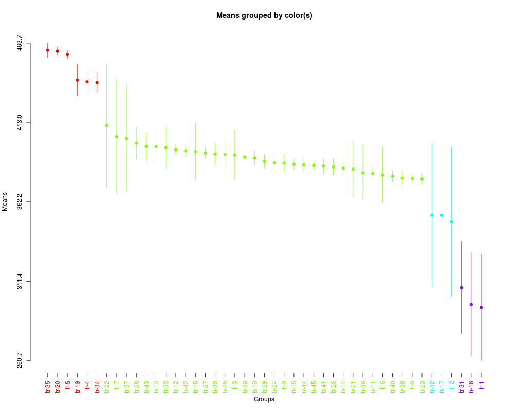
> summary(sk2)
Levels Means SK(5%)
tr-35 459.1650 a
tr-20 458.5300 a
tr-5 456.3500 a
tr-19 440.0750 a
tr-4 438.9850 a
tr-34 438.4225 a
tr-22 410.9100 b
tr-7 403.8800 b
tr-37 402.5925 b
tr-28 399.6675 b
tr-43 397.6000 b
tr-13 397.5025 b
tr-33 396.8950 b
tr-12 395.4875 b
tr-42 394.7650 b
tr-18 394.2600 b
tr-27 393.3200 b
tr-39 392.8200 b
tr-25 392.4100 b
tr-3 392.0725 b
tr-30 390.7950 b
tr-10 390.2025 b
tr-29 388.1975 b
tr-24 387.1950 b
tr-9 386.9500 b
tr-15 386.2050 b
tr-44 385.8675 b
tr-45 385.3325 b
tr-41 384.9825 b
tr-26 384.4675 b
tr-14 383.6075 b
tr-21 383.0625 b
tr-36 380.7450 b
tr-11 380.3875 b
tr-6 379.3175 b
tr-40 378.5675 b
tr-38 377.3475 b
tr-8 377.0425 b
tr-23 376.8125 b
tr-32 353.7575 c
tr-17 353.6525 c
tr-2 349.3500 c
tr-31 307.3700 d
tr-16 296.6125 d
tr-1 294.6800 d
> plot(sk2,
+ col=rainbow(max(sk2$groups)),
+ id.las=2,
+ rl=FALSE)
>
> ## From: aov
> av <- with(CRD2,
+ aov(y ~ x,
+ data=dfm))
> summary(av)
Df Sum Sq Mean Sq F value Pr(>F)
x 44 209136 4753 3.273 7.69e-08 ***
Residuals 135 196045 1452
---
Signif. codes: 0 '***' 0.001 '**' 0.01 '*' 0.05 '.' 0.1 ' ' 1
>
> sk3 <- SK(x=av,
+ which='x')
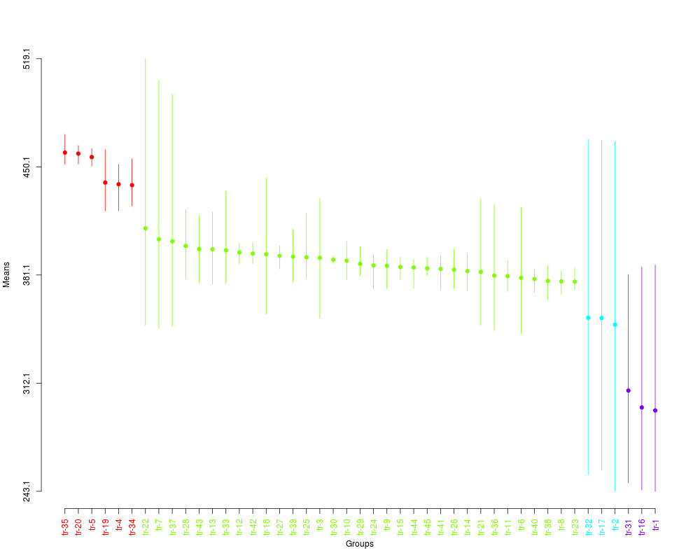
> summary(sk3)
Levels Means SK(5%)
tr-35 459.1650 a
tr-20 458.5300 a
tr-5 456.3500 a
tr-19 440.0750 a
tr-4 438.9850 a
tr-34 438.4225 a
tr-22 410.9100 b
tr-7 403.8800 b
tr-37 402.5925 b
tr-28 399.6675 b
tr-43 397.6000 b
tr-13 397.5025 b
tr-33 396.8950 b
tr-12 395.4875 b
tr-42 394.7650 b
tr-18 394.2600 b
tr-27 393.3200 b
tr-39 392.8200 b
tr-25 392.4100 b
tr-3 392.0725 b
tr-30 390.7950 b
tr-10 390.2025 b
tr-29 388.1975 b
tr-24 387.1950 b
tr-9 386.9500 b
tr-15 386.2050 b
tr-44 385.8675 b
tr-45 385.3325 b
tr-41 384.9825 b
tr-26 384.4675 b
tr-14 383.6075 b
tr-21 383.0625 b
tr-36 380.7450 b
tr-11 380.3875 b
tr-6 379.3175 b
tr-40 378.5675 b
tr-38 377.3475 b
tr-8 377.0425 b
tr-23 376.8125 b
tr-32 353.7575 c
tr-17 353.6525 c
tr-2 349.3500 c
tr-31 307.3700 d
tr-16 296.6125 d
tr-1 294.6800 d
> plot(sk3,
+ col=rainbow(max(sk3$groups)),
+ rl=FALSE,
+ id.las=2,
+ title=NULL)
>
> ##
> ## Example: Randomized Complete Block Design (RCBD)
> ## More details: demo(package='ScottKnott')
> ##
>
> ## The parameters can be: design matrix and the response variable,
> ## data.frame or aov
>
> data(RCBD)
>
> ## Design matrix (dm) and response variable (y)
> sk1 <- with(RCBD,
+ SK(x=dm,
+ y=y,
+ model='y ~ blk + tra',
+ which='tra'))
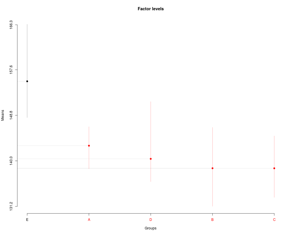
> summary(sk1)
Levels Means SK(5%)
E 155.3700 a
A 142.9325 b
D 140.3950 b
B 138.5750 b
C 138.5650 b
> plot(sk1)
>
> ## From: data.frame (dfm), which='tra'
> sk2 <- with(RCBD,
+ SK(x=dfm,
+ model='y ~ blk + tra',
+ which='tra'))
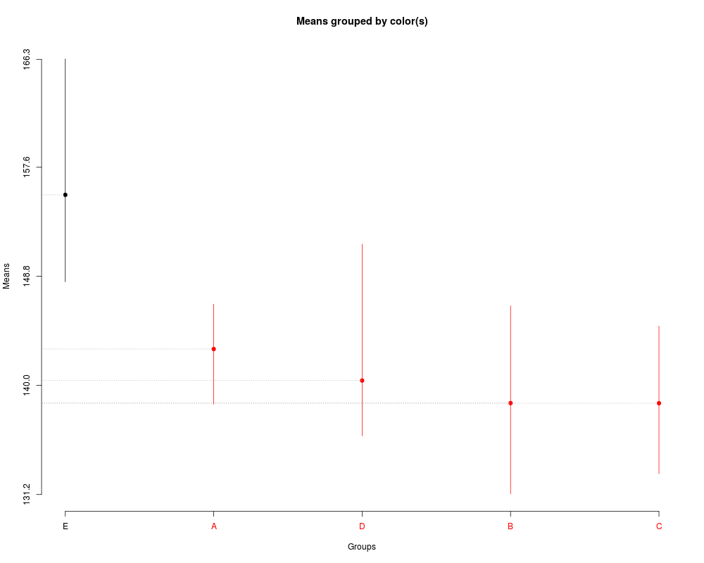
> summary(sk2)
Levels Means SK(5%)
E 155.3700 a
A 142.9325 b
D 140.3950 b
B 138.5750 b
C 138.5650 b
> plot(sk2,
+ mm.lty=3,
+ title='Factor levels')
>
> ##
> ## Example: Latin Squares Design (LSD)
> ## More details: demo(package='ScottKnott')
> ##
>
> ## The parameters can be: design matrix and the response variable,
> ## data.frame or aov
>
> data(LSD)
>
> ## From: design matrix (dm) and response variable (y)
> sk1 <- with(LSD,
+ SK(x=dm,
+ y=y,
+ model='y ~ rows + cols + tra',
+ which='tra'))
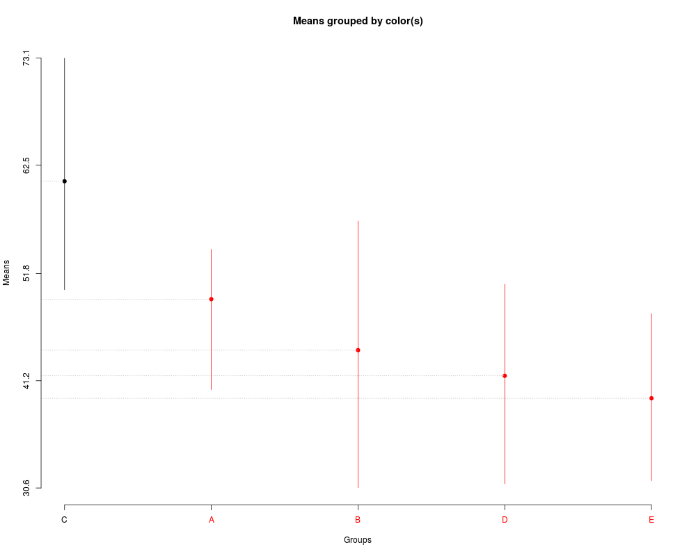
> summary(sk1)
Levels Means SK(5%)
C 60.910 a
A 49.258 b
B 44.216 b
D 41.686 b
E 39.464 b
> plot(sk1)
>
> ## From: data.frame
> sk2 <- with(LSD,
+ SK(x=dfm,
+ model='y ~ rows + cols + tra',
+ which='tra'))
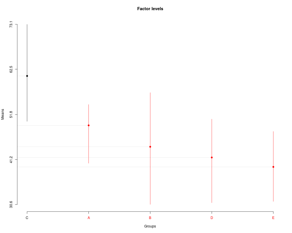
> summary(sk2)
Levels Means SK(5%)
C 60.910 a
A 49.258 b
B 44.216 b
D 41.686 b
E 39.464 b
> plot(sk2,
+ title='Factor levels')
>
> ## From: aov
> av <- with(LSD,
+ aov(y ~ rows + cols + tra,
+ data=dfm))
> summary(av)
Df Sum Sq Mean Sq F value Pr(>F)
rows 4 398.8 99.7 4.193 0.023679 *
cols 4 589.9 147.5 6.201 0.006059 **
tra 4 1456.6 364.1 15.313 0.000116 ***
Residuals 12 285.4 23.8
---
Signif. codes: 0 '***' 0.001 '**' 0.01 '*' 0.05 '.' 0.1 ' ' 1
>
> sk3 <- SK(av,
+ which='tra')
> summary(sk3)
Levels Means SK(5%)
C 60.910 a
A 49.258 b
B 44.216 b
D 41.686 b
E 39.464 b
> plot(sk3,
+ title='Factor levels')
>
> ##
> ## Example: Factorial Experiment (FE)
> ## More details: demo(package='ScottKnott')
> ##
>
> ## The parameters can be: design matrix and the response variable,
> ## data.frame or aov
>
> ## Note: The factors are in uppercase and its levels in lowercase!
>
> data(FE)
>
> ## From: design matrix (dm) and response variable (y)
> ## Main factor: N
> sk1 <- with(FE,
+ SK(x=dm,
+ y=y,
+ model='y ~ blk + N*P*K',
+ which='N'))
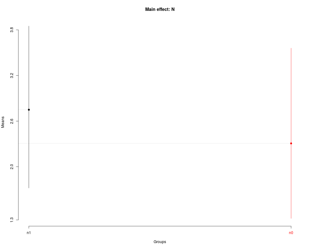
> summary(sk1)
Levels Means SK(5%)
n1 2.750000 a
n0 2.306875 b
> plot(sk1,
+ title='Main effect: N')
>
> ## Nested: p1/N
> ## Studing N inside of level one of P
> nsk1 <- with(FE,
+ SK.nest(x=dm,
+ y=y,
+ model='y ~ blk + N*P*K',
+ which='P:N',
+ fl1=1))
> summary(nsk1)
Nested: N/P
Levels Means SK(5%)
p0/n1 2.60375 a
p0/n0 2.41125 a
> plot(nsk1,
+ title='Effect: p1/N')
>
> ## Nested: k1/P
> nsk2 <- with(FE,
+ SK.nest(x=dm,
+ y=y,
+ model='y ~ blk + N*P*K',
+ which='K:P',
+ fl1=1))
> summary(nsk2)
Nested: P/K
Levels Means SK(5%)
k0/p1 2.47750 a
k0/p0 2.18125 a
> plot(nsk2,
+ title='Effect: k1/P')
>
> ## Nested: k2/p2/N
> nsk3 <- with(FE,
+ SK.nest(x=dm,
+ y=y,
+ model='y ~ blk + N*P*K',
+ which='K:P:N',
+ fl1=2,
+ fl2=2))
> summary(nsk3)
Nested: N/P/K
Levels Means SK(5%)
k1/p1/n1 2.9950 a
k1/p1/n0 2.2475 b
> plot(nsk3,
+ title='Effect: k2/p2/N')
>
> ## Nested: k1/n1/P
> ## Studing P inside of level one of K and level one of N
> nsk4 <- with(FE,
+ SK.nest(x=dm,
+ y=y,
+ model='y ~ blk + N*P*K',
+ which='K:N:P',
+ fl1=1,
+ fl2=1))
> summary(nsk4)
Nested: N/P/K
Levels Means SK(5%)
k0/n0/p1 2.1575 a
k0/n0/p0 1.8850 a
> plot(nsk4,
+ title='Effect: k1/n1/P')
>
> ## Nested: p1/n1/K
> nsk5 <- with(FE,
+ SK.nest(x=dm,
+ y=y,
+ model='y ~ blk + N*P*K',
+ which='P:N:K',
+ fl1=1,
+ fl2=1))
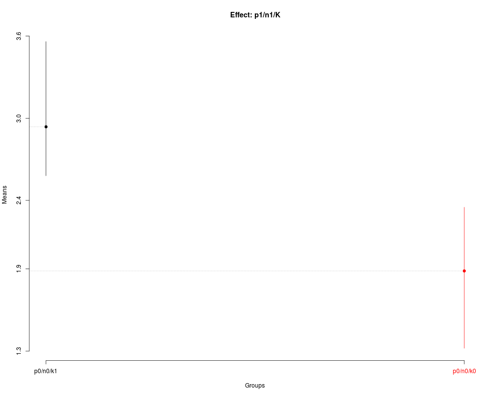
> summary(nsk5)
Nested: N/P/K
Levels Means SK(5%)
p0/n0/k1 2.9375 a
p0/n0/k0 1.8850 b
> plot(nsk5, title='Effect: p1/n1/K')
>
> ##
> ## Example: Split-plot Experiment (SPE)
> ## More details: demo(package='ScottKnott')
> ##
>
> ## Note: The factors are in uppercase and its levels in lowercase!
>
> data(SPE)
>
> ## The parameters can be: design matrix and the response variable,
> ## data.frame or aov
>
> ## From: design matrix (dm) and response variable (y)
> ## Main factor: P
> sk1 <- with(SPE,
+ SK(x=dm,
+ y=y,
+ model='y ~ blk + P*SP + Error(blk/P)',
+ which='P',
+ error='blk:P'))
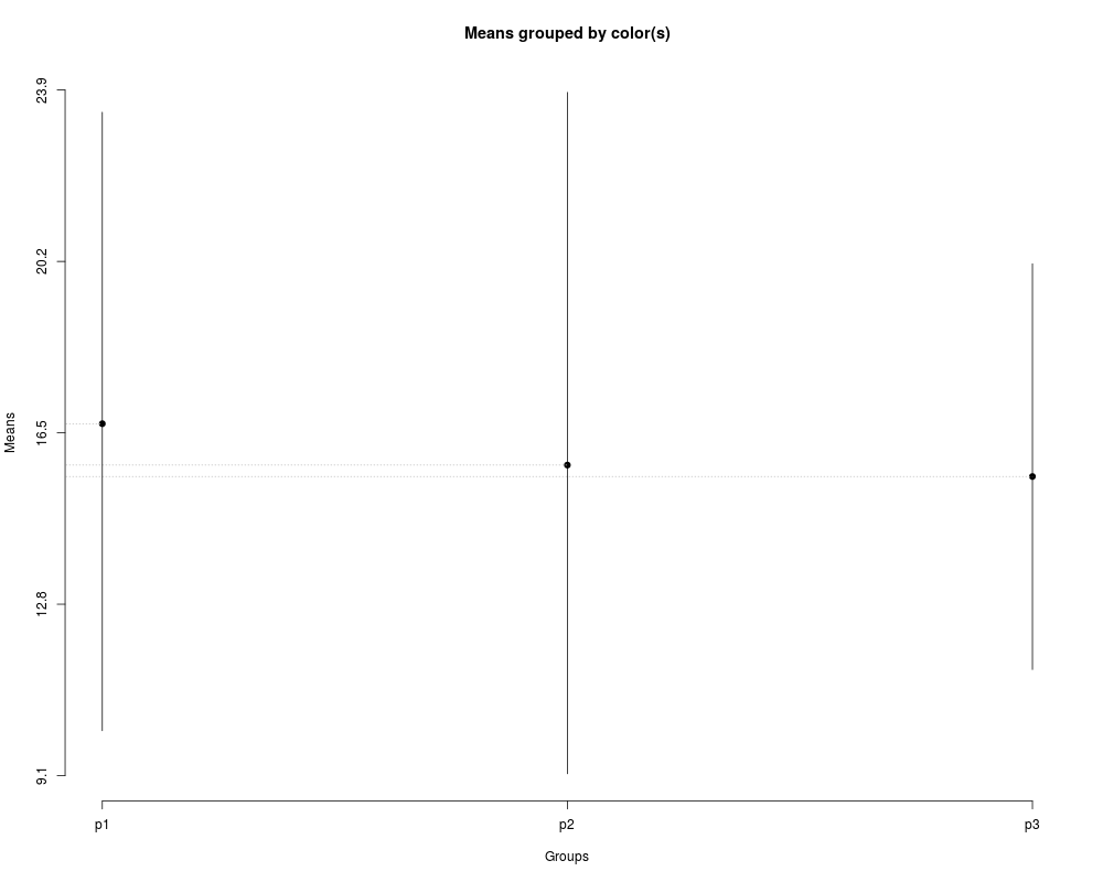
> summary(sk1)
Levels Means SK(5%)
p1 16.69667 a
p2 15.80417 a
p3 15.55667 a
> plot(sk1)
>
> ## Main factor: SP
> sk2 <- with(SPE,
+ SK(x=dm,
+ y=y,
+ model='y ~ blk + P*SP + Error(blk/P)',
+ which='SP',
+ error='Within'))
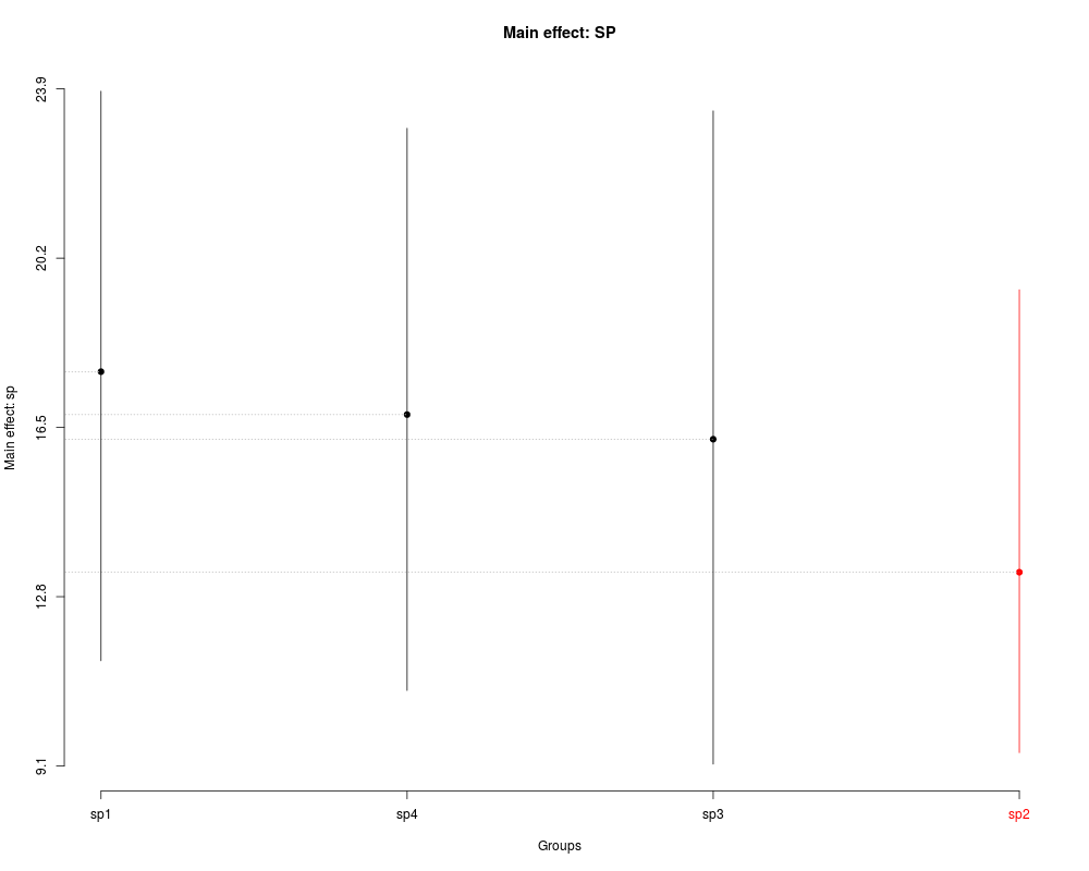
> summary(sk2)
Levels Means SK(5%)
sp1 17.71833 a
sp4 16.78056 a
sp3 16.24278 a
sp2 13.33500 b
> plot(sk2,
+ xlab='Groups',
+ ylab='Main effect: sp',
+ title='Main effect: SP')
>
> ## Nested: p1/SP
> skn1 <- with(SPE,
+ SK.nest(x=dm,
+ y=y,
+ model='y ~ blk + P*SP + Error(blk/P)',
+ which='P:SP',
+ error='Within',
+ fl1=1 ))
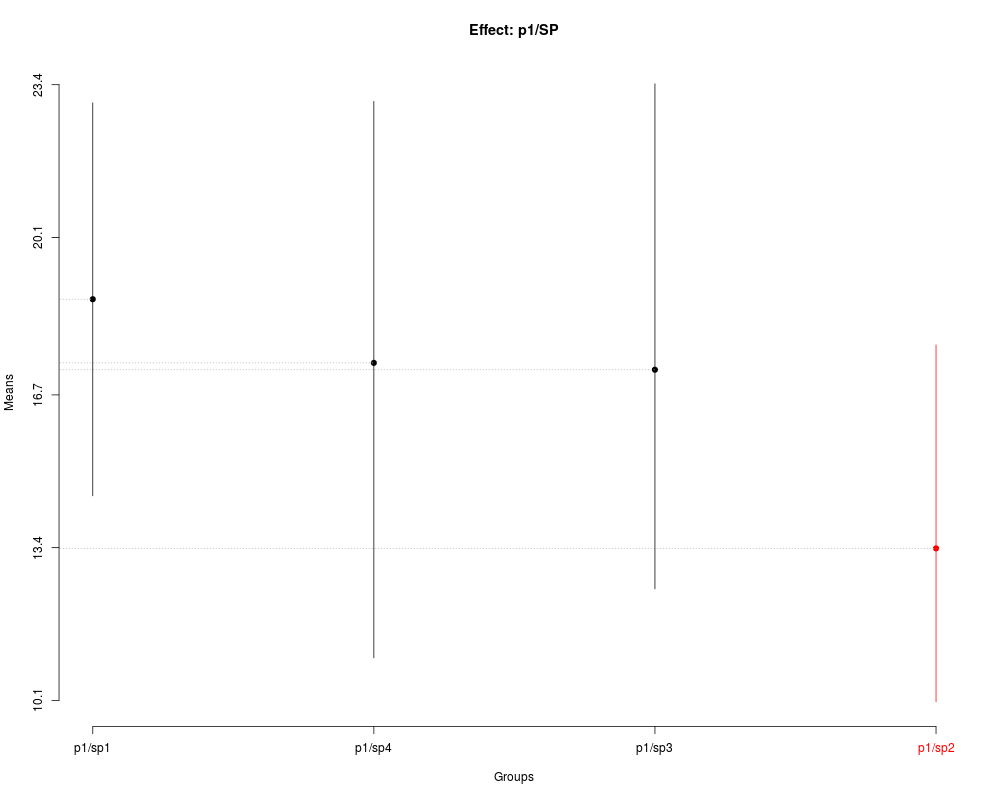
> summary(skn1)
Nested: P/SP
Levels Means SK(5%)
p1/sp1 18.76667 a
p1/sp4 17.39167 a
p1/sp3 17.24333 a
p1/sp2 13.38500 b
> plot(skn1,
+ title='Effect: p1/SP')
>
> ##
> ## Example: Split-split-plot Experiment (SSPE)
> ## More details: demo(package='ScottKnott')
> ##
>
> ## Note: The factors are in uppercase and its levels in lowercase!
>
> data(SSPE)
>
> ## From: design matrix (dm) and response variable (y)
> ## Main factor: P
> sk1 <- with(SSPE,
+ SK(dm,
+ y,
+ model='y ~ blk + P*SP*SSP + Error(blk/P/SP)',
+ which='P',
+ error='blk:P'))
> summary(sk1)
Levels Means SK(5%)
p2 389.9978 a
p3 389.0820 a
p1 387.4680 a
>
> # Main factor: SP
> sk2 <- with(SSPE,
+ SK(dm,
+ y,
+ model='y ~ blk + P*SP*SSP + Error(blk/P/SP)',
+ which='SP',
+ error='blk:P:SP'))
> summary(sk2)
Levels Means SK(5%)
sp3 389.8790 a
sp1 388.6785 a
sp2 387.9903 a
>
> # Main factor: SSP
> sk3 <- with(SSPE,
+ SK(dm,
+ y,
+ model='y ~ blk + P*SP*SSP + Error(blk/P/SP)',
+ which='SSP',
+ error='Within'))
> summary(sk3)
Levels Means SK(5%)
ssp5 410.8397 a
ssp4 404.6800 a
ssp3 389.9111 b
ssp2 384.1906 b
ssp1 354.6250 c
>
> ## Nested: p1/SP
> skn1 <- with(SSPE,
+ SK.nest(dm,
+ y,
+ model='y ~ blk + P*SP*SSP + Error(blk/P/SP)',
+ which='P:SP',
+ error='blk:P:SP',
+ fl1=1))
> summary(skn1)
Nested: P/SP
Levels Means SK(5%)
p1/sp3 388.6380 a
p1/sp2 387.4785 a
p1/sp1 386.2875 a
>
> ## From: aovlist
> av <- with(SSPE,
+ aov(y ~ blk + P*SP*SSP + Error(blk/P/SP),
+ data=dfm))
> summary(av)
Error: blk
Df Sum Sq Mean Sq
blk 3 15692 5231
Error: blk:P
Df Sum Sq Mean Sq F value Pr(>F)
P 2 196.9 98.44 1.368 0.324
Residuals 6 431.7 71.94
Error: blk:P:SP
Df Sum Sq Mean Sq F value Pr(>F)
SP 2 110 54.8 0.113 0.894
P:SP 4 250 62.5 0.129 0.970
Residuals 18 8735 485.3
Error: Within
Df Sum Sq Mean Sq F value Pr(>F)
SSP 4 69420 17355 10.949 1.72e-07 ***
P:SSP 8 392 49 0.031 1
SP:SSP 8 138209 17276 10.899 3.68e-11 ***
P:SP:SSP 16 559 35 0.022 1
Residuals 108 171186 1585
---
Signif. codes: 0 '***' 0.001 '**' 0.01 '*' 0.05 '.' 0.1 ' ' 1
>
> ## Nested: p/sp/SSP (at various levels of sp and p)
> skn6 <- SK.nest(av,
+ which='P:SP:SSP',
+ error='Within',
+ fl1=1,
+ fl2=1)
> summary(skn6)
Nested: P/SP/SSP
Levels Means SK(5%)
p1/sp1/ssp5 456.3500 a
p1/sp1/ssp4 438.9850 a
p1/sp1/ssp3 392.0725 a
p1/sp1/ssp2 349.3500 b
p1/sp1/ssp1 294.6800 b
>
> skn7 <- SK.nest(av,
+ which='P:SP:SSP',
+ error='Within',
+ fl1=2,
+ fl2=1)
> summary(skn7)
Nested: P/SP/SSP
Levels Means SK(5%)
p2/sp1/ssp5 458.5300 a
p2/sp1/ssp4 440.0750 a
p2/sp1/ssp3 394.2600 a
p2/sp1/ssp2 353.6525 b
p2/sp1/ssp1 296.6125 c
>
>
>
>
>
> dev.off()
null device
1
>
|