R Graphical Manual

Browse All

Last data update: 2014.03.03

R: Plot SK and SK.nest Objects

plot.SK

R Documentation

Plot SK and SK.nest Objects

Description

S3 method to plot SK and SK.nest objects.

Usage

## S3 method for class 'SK'
plot(x,
     pch=19, 
     col=NULL,
     xlab=NULL,
     ylab=NULL,
     xlim=NULL,
     ylim=NULL,
     id.lab=NULL,
     id.las=1,
     id.col=TRUE,
     rl=TRUE,
     rl.lty=3,
     rl.col='gray',
     mm=TRUE,
     mm.lty=1, 
     title="Means grouped by color(s)", ...)

Arguments

`x`	A `SK` object.
`pch`	A vector of plotting symbols or characters.
`col`	A vector of colors for the means representation.
`xlab`	A label for the x axis.
`ylab`	A label for the y axis.
`xlim`	The x limits of the plot.
`ylim`	The y limits of the plot.
`id.lab`	Factor level names at x-axis.
`id.las`	Factor level names written either horizontally or vertically.
`id.col`	A logical value. If `TRUE` (the default), the `col` parameter will be used for the x axis.
`rl`	Horizontal line connecting the circle to the y-axis.
`rl.lty`	Line type of rl.
`rl.col`	Line color of rl.
`mm`	Vertical line through the circle (mean value) linking the minimum to the maximum of the factor level values corresponding to that mean value.
`mm.lty`	Line type of mm.
`title`	A title for the plot.
`...`	Optional plotting parameters.

Details

The plot.SK function is a S3 method to plot SK and SK.nest objetcs. It generates a serie of points (the means) and a vertical line showing the minimum e maximum of the values corresponding to each group mean. The groups are diferentiated by colors.

Author(s)

Enio Jelihovschi (eniojelihovs@gmail.com)
Jos<c3><a9> Cl<c3><a1>udio Faria (joseclaudio.faria@gmail.com)
Ivan Bezerra Allaman (ivanalaman@gmail.com)

References

Murrell, P. 2005. R Graphics. Chapman & Hall/CRC Press.

Examples

##
## Examples: Completely Randomized Design (CRD)
## More details: demo(package='ScottKnott')
##

library(ScottKnott)
data(CRD2)

## From: vectors x and y
sk1 <- with(CRD2,
            SK(x=x,
               y=y,
               model='y ~ x',
               which='x'))

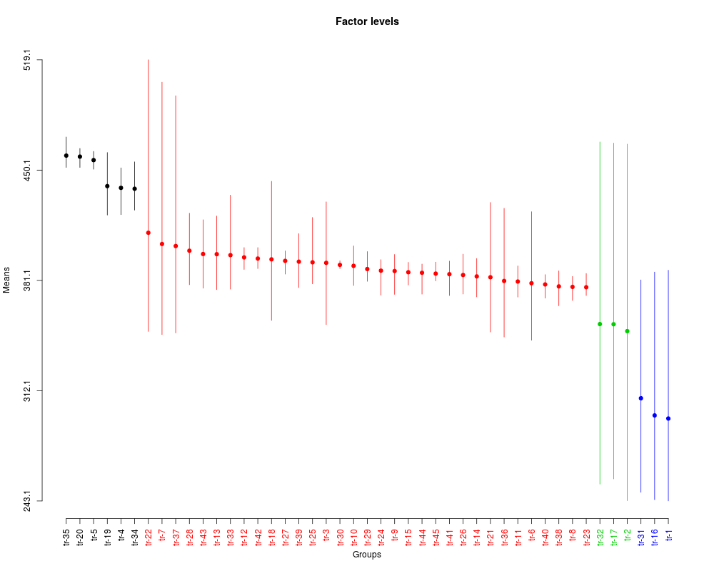
plot(sk1,
     id.las=2,
     rl=FALSE, 
     title='Factor levels')

## From: design matrix (dm) and response variable (y)
sk2 <- with(CRD2,
            SK(x=dm,
               y=y,
               model='y ~ x',
               which='x'))
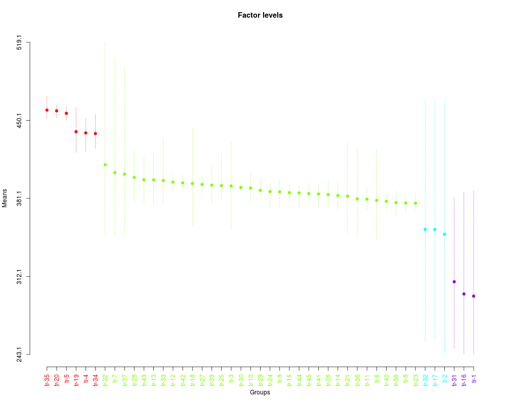
plot(sk2,
     col=rainbow(max(sk2$groups)),
     mm.lty=3,
     id.las=2,
     rl=FALSE,
     title='Factor levels')

## From: data.frame (dfm)
sk3 <- with(CRD2,
            SK(x=dfm,
               model='y ~ x',
               which='x'))

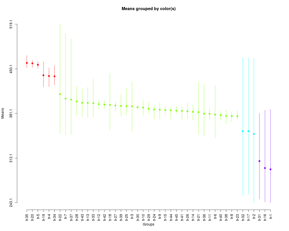
plot(sk3,
     col=rainbow(max(sk3$groups)),
     id.las=2,
     id.col=FALSE,
     rl=FALSE)

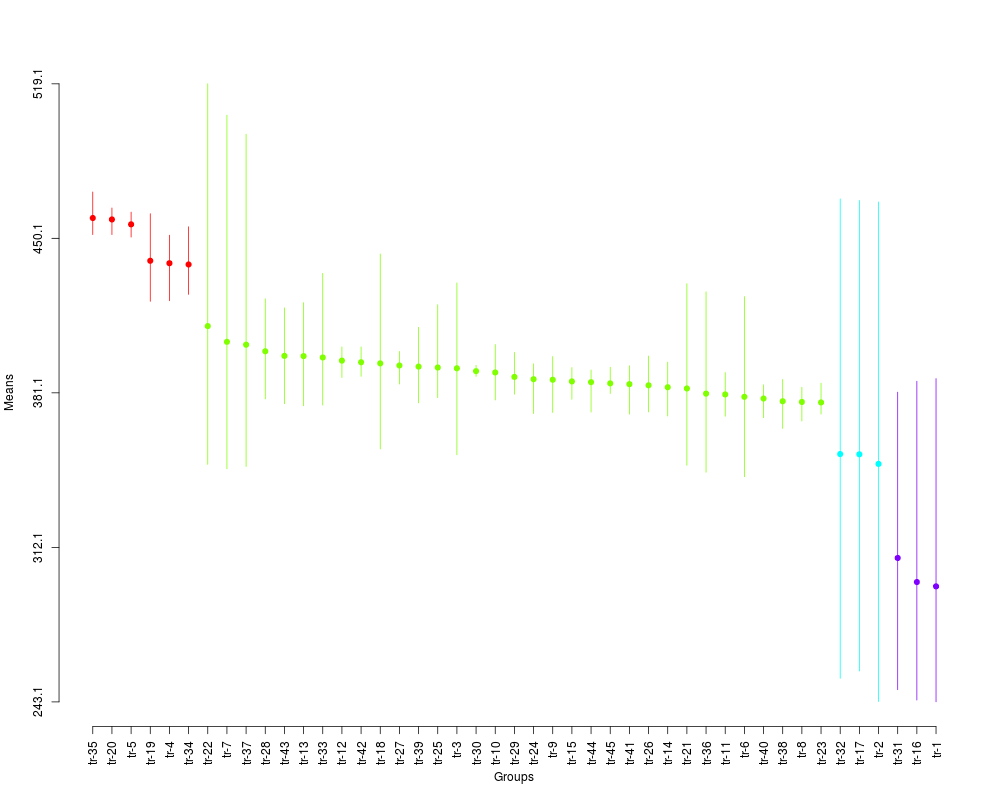
## From: aov
av <- with(CRD2,
           aov(y ~ x,
               data=dfm))
summary(av)

sk4 <- with(CRD2,
            SK(x=av,
               which='x'))

plot(sk4,
     col=rainbow(max(sk4$groups)),
     rl=FALSE,
     id.las=2,
     id.col=FALSE,
     title=NULL)

Results


R version 3.3.1 (2016-06-21) -- "Bug in Your Hair"
Copyright (C) 2016 The R Foundation for Statistical Computing
Platform: x86_64-pc-linux-gnu (64-bit)

R is free software and comes with ABSOLUTELY NO WARRANTY.
You are welcome to redistribute it under certain conditions.
Type 'license()' or 'licence()' for distribution details.

R is a collaborative project with many contributors.
Type 'contributors()' for more information and
'citation()' on how to cite R or R packages in publications.

Type 'demo()' for some demos, 'help()' for on-line help, or
'help.start()' for an HTML browser interface to help.
Type 'q()' to quit R.

> library(ScottKnott)
> png(filename="/home/ddbj/snapshot/RGM3/R_CC/result/ScottKnott/plot.SK.Rd_%03d_medium.png", width=480, height=480)
> ### Name: plot.SK
> ### Title: Plot SK and SK.nest Objects
> ### Aliases: plot.SK
> ### Keywords: package htest univar tree design
> 
> ### ** Examples
> 
> ##
> ## Examples: Completely Randomized Design (CRD)
> ## More details: demo(package='ScottKnott')
> ##
> 
> library(ScottKnott)
> data(CRD2)
> 
> ## From: vectors x and y
> sk1 <- with(CRD2,
+             SK(x=x,
+                y=y,
+                model='y ~ x',
+                which='x'))
> 
> plot(sk1,
+      id.las=2,
+      rl=FALSE, 
+      title='Factor levels')
> 
> ## From: design matrix (dm) and response variable (y)
> sk2 <- with(CRD2,
+             SK(x=dm,
+                y=y,
+                model='y ~ x',
+                which='x'))
> plot(sk2,
+      col=rainbow(max(sk2$groups)),
+      mm.lty=3,
+      id.las=2,
+      rl=FALSE,
+      title='Factor levels')
> 
> ## From: data.frame (dfm)
> sk3 <- with(CRD2,
+             SK(x=dfm,
+                model='y ~ x',
+                which='x'))
> 
> plot(sk3,
+      col=rainbow(max(sk3$groups)),
+      id.las=2,
+      id.col=FALSE,
+      rl=FALSE)
> 
> ## From: aov
> av <- with(CRD2,
+            aov(y ~ x,
+                data=dfm))
> summary(av)
             Df Sum Sq Mean Sq F value   Pr(>F)    
x            44 209136    4753   3.273 7.69e-08 ***
Residuals   135 196045    1452                     
---
Signif. codes:  0 '***' 0.001 '**' 0.01 '*' 0.05 '.' 0.1 ' ' 1
> 
> sk4 <- with(CRD2,
+             SK(x=av,
+                which='x'))
> 
> plot(sk4,
+      col=rainbow(max(sk4$groups)),
+      rl=FALSE,
+      id.las=2,
+      id.col=FALSE,
+      title=NULL)
> 
> 
> 
> 
> 
> dev.off()
null device 
          1 
>