Fitting Contamination Model

Description

Provides ML estimates of a Gaussian contamination model.

Usage

    ml.est (y, x=NULL, model = "LN", lambda=3,  w=0.05,
            lambda.fix=FALSE, w.fix=FALSE, eps=1e-7,  
            max.iter=500, t.outl=0.5, graph=FALSE)

Arguments

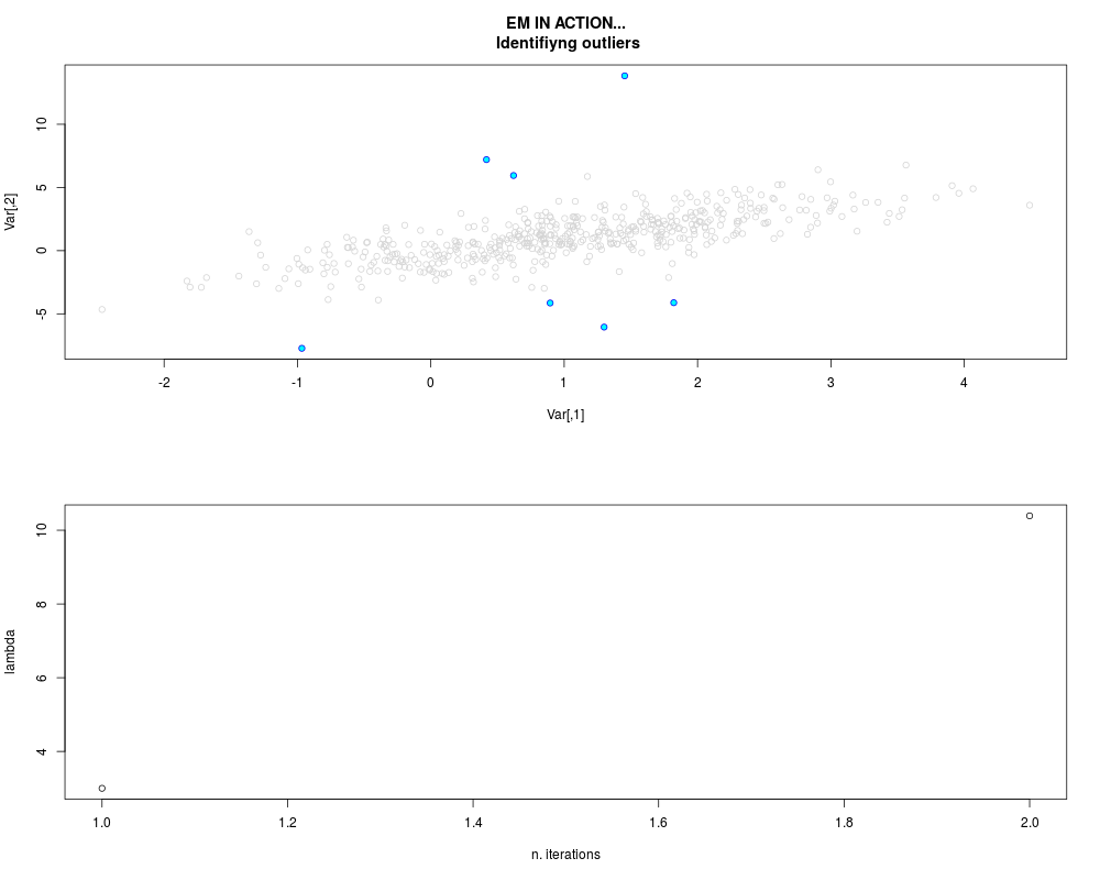
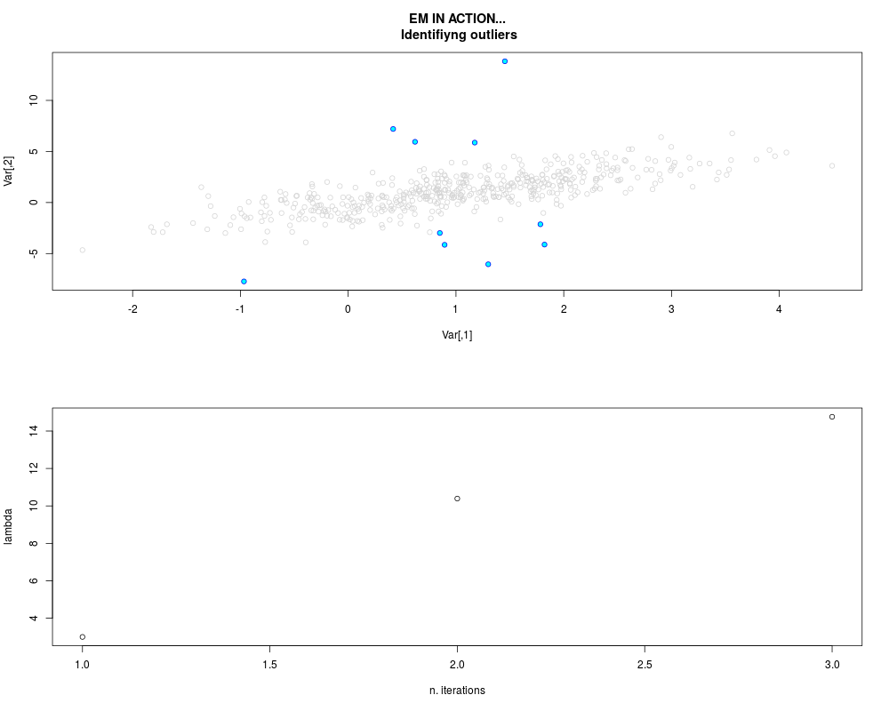
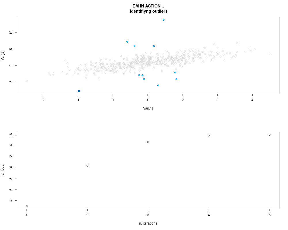
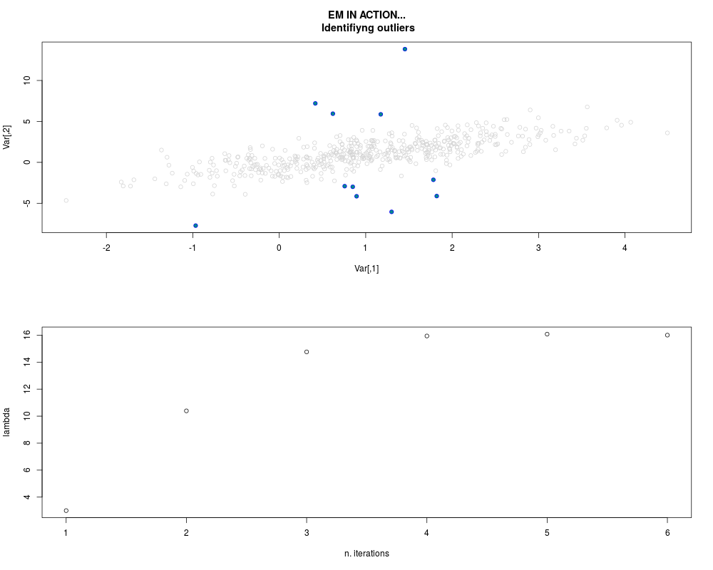
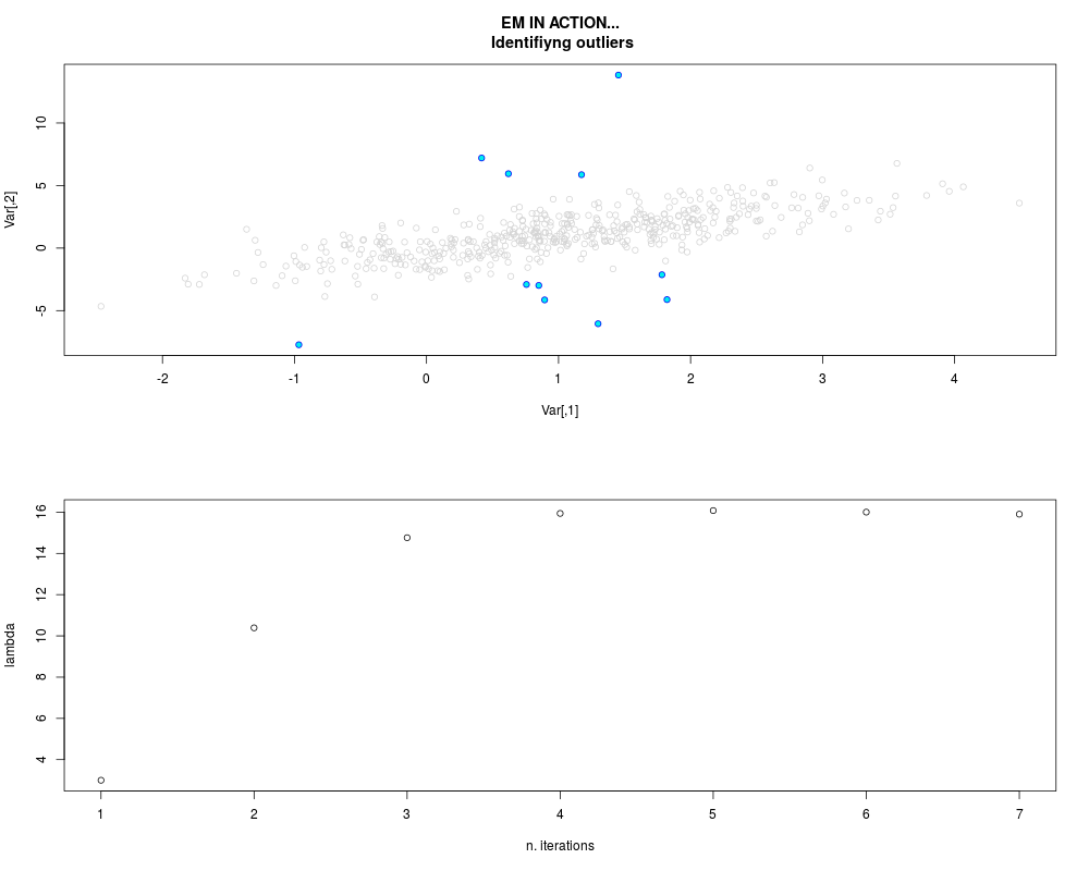
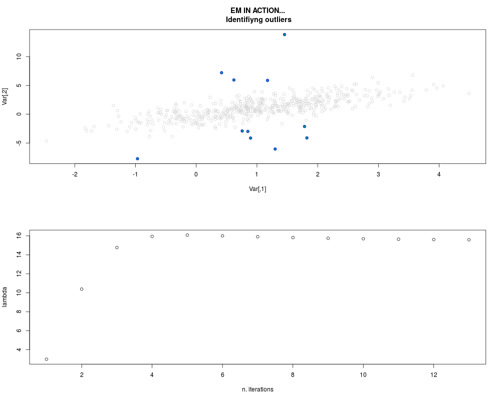
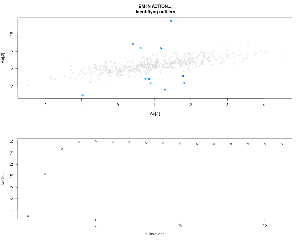
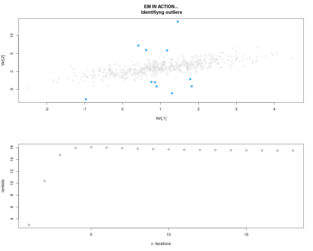
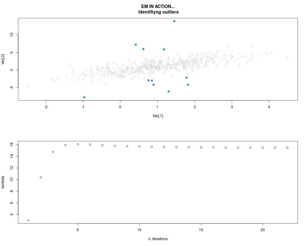
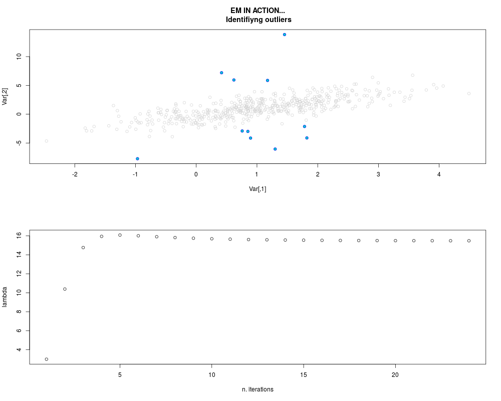
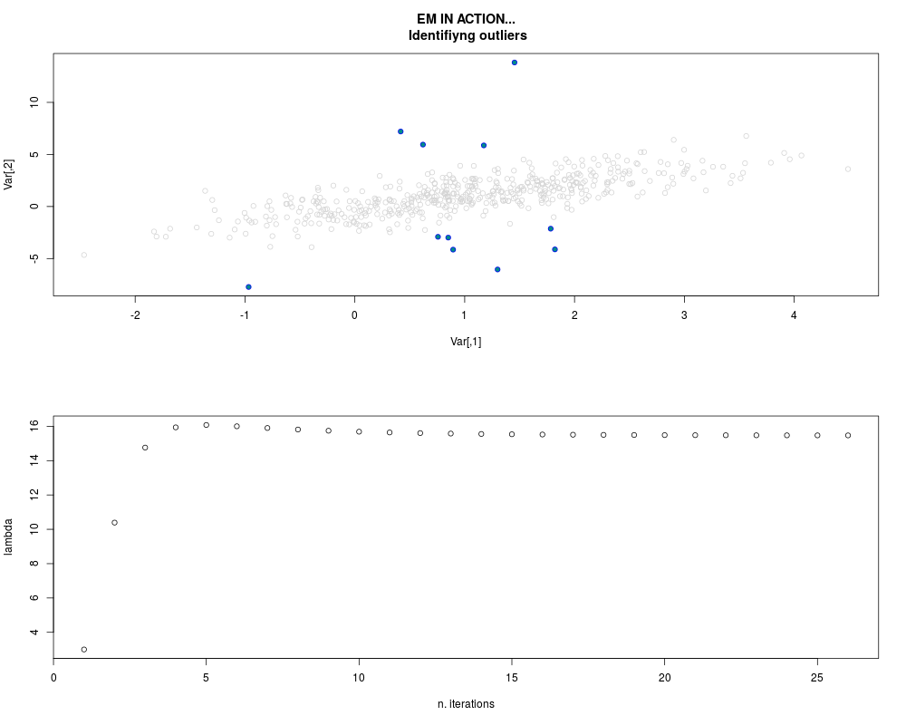
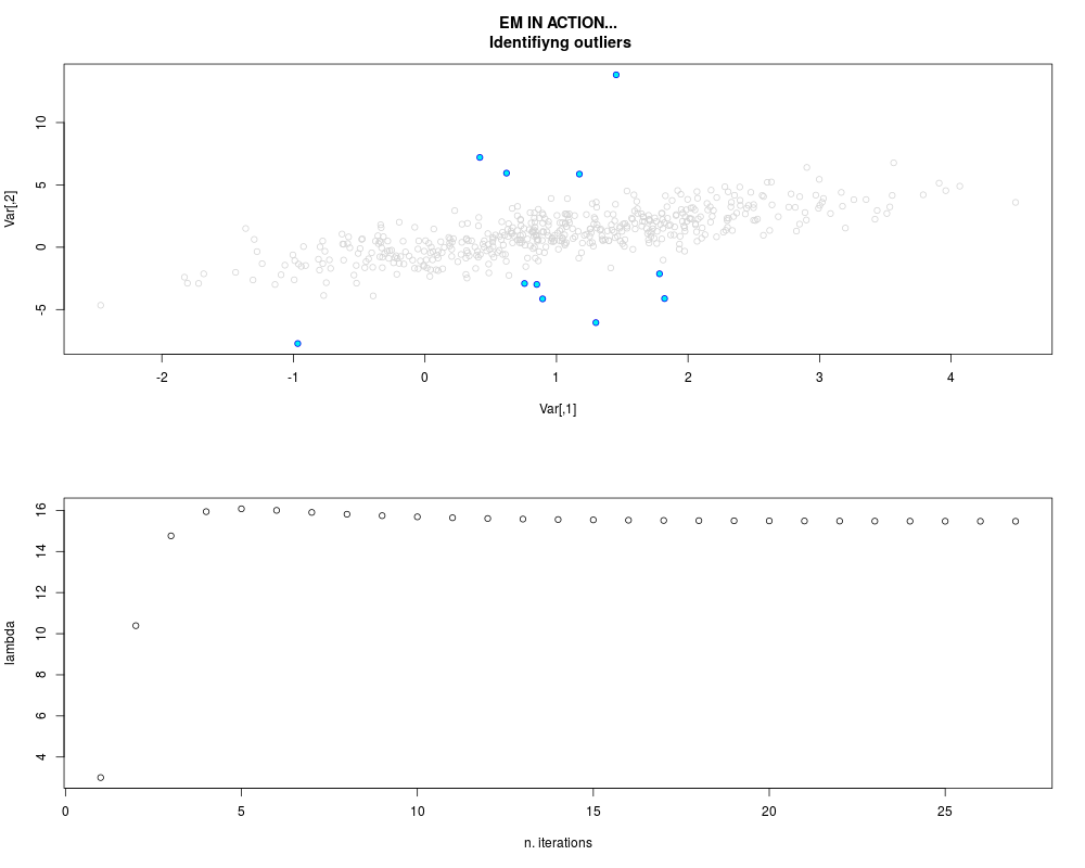
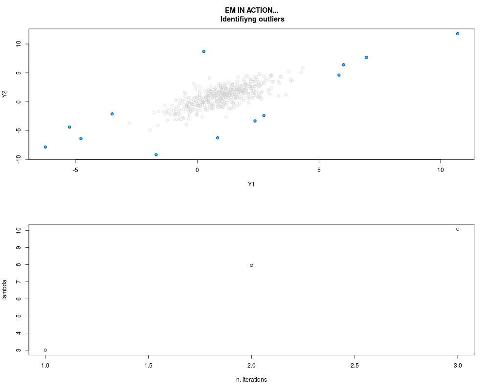
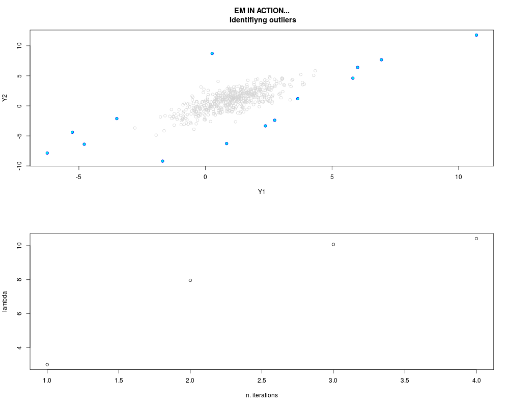
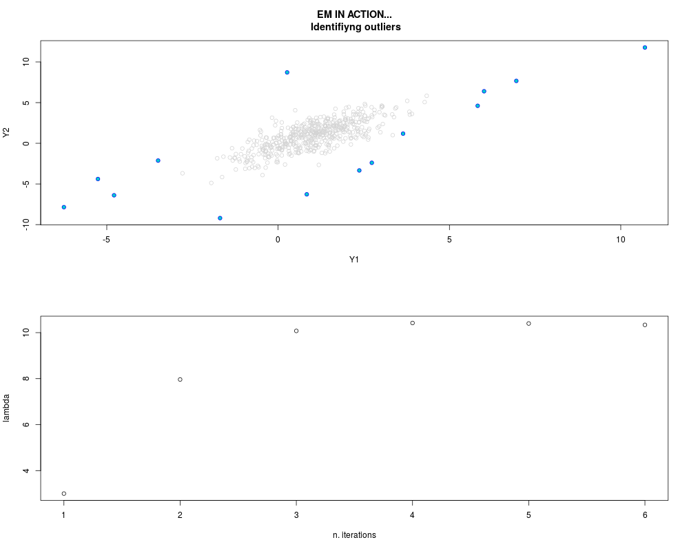
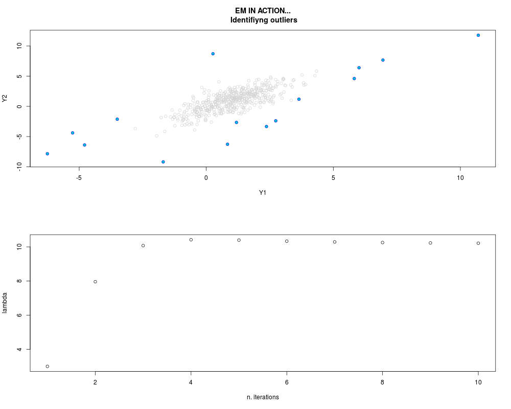
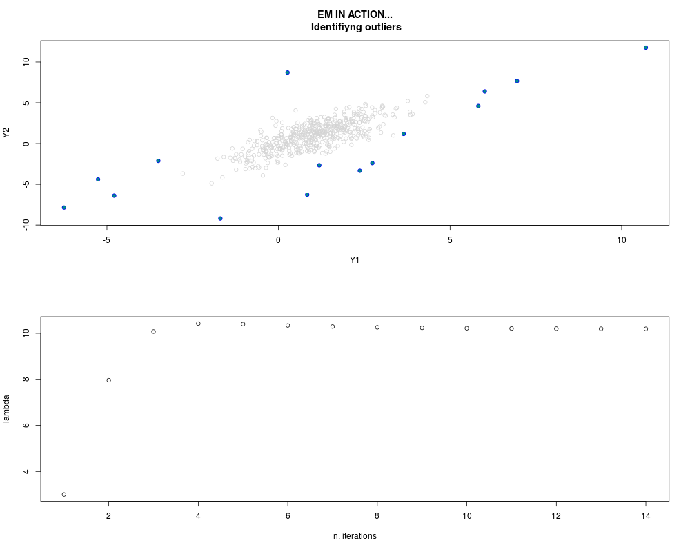
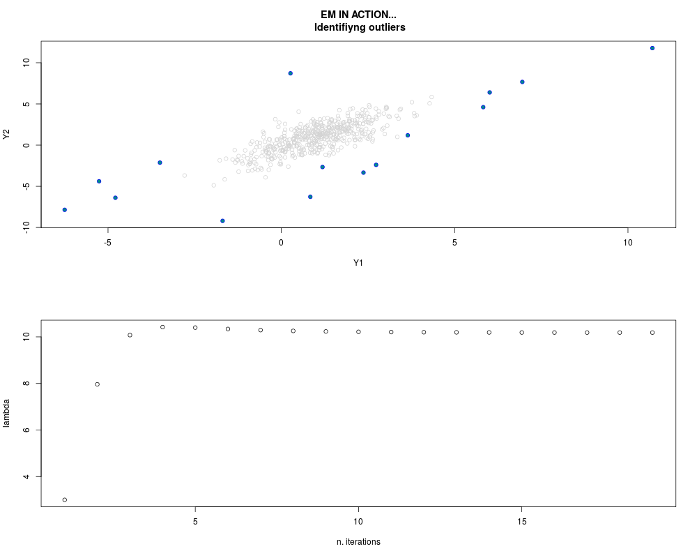
Details

This function provides the parameter estimates of a contamination model where a set of y variables is assumed to depend on a (possibly empty) set of covariates (x variables) through a mixture of two linear regressions with Gaussian residuals. The covariance matrices of the two mixture components are assumed to be proportional (the proportionality constant being lambda). In case of no x variables a mixture of two Gaussian distribution is estimated. BIC and AIC scores (bic.aic) are returned corresponding to both standard Gaussian model and contamination model in order to help the user to avoid possible over-parametrisation.

According to the estimated model parameters, a matrix of predictions of ‘true’ y values (ypred) is computed. To each unit in the dataset, a flag (outlier) is assigned taking value 0 or 1 depending on whether the posterior probability of being erroneous (tau) is greater than the user specified threshold (t.outl).

The model is estimated using complete observations. Missing values in the x variables are not allowed. However, y variables can be partly observed. Robust predictions of y variables are provided even when they are not observed. A vector of missing pattern (pattern) indicates which item is observed and which is missing.

In case the option ‘model = LN’ is specified, each zero value is changed in 1e-7 and a warning is returned.

In order to graphically monitor EM algorithm, a scatter plot is showed where outliers are depicted as long as they are identified. The trajectory of the lambda parameter is also showed until convergence.

Value

ml.est returns a list containing the following components:

Author(s)

M. Teresa Buglielli <bugliell@istat.it>, Ugo Guarnera <guarnera@istat.it>

References

Di Zio, M., Guarnera, U. (2013) "A Contamination Model for Selective Editing", Journal of Official Statistics. Volume 29, Issue 4, Pages 539-555 (http://dx.doi.org/10.2478/jos-2013-0039).

Buglielli, M.T., Di Zio, M., Guarnera, U. (2010) "Use of Contamination Models for Selective Editing", European Conference on Quality in Survey Statistics Q2010, Helsinki, 4-6 May 2010

Examples

# Parameter estimation with one contaminated variable and one covariate
        data(ex1.data)
        ml.par <- ml.est(y=ex1.data[,"Y1"], x=ex1.data[,"X1"], graph=TRUE) 
        str(ml.par)
        sum(ml.par$outlier)  # number of outliers
# Parameter estimation with two contaminated variables and no covariates
        data(ex2.data)
        par.joint <- ml.est(y=ex2.data, x=NULL, graph=TRUE)  
        sum(par.joint$outlier)  # number of outliers           

Results

R version 3.3.1 (2016-06-21) -- "Bug in Your Hair"
Copyright (C) 2016 The R Foundation for Statistical Computing
Platform: x86_64-pc-linux-gnu (64-bit)

R is free software and comes with ABSOLUTELY NO WARRANTY.
You are welcome to redistribute it under certain conditions.
Type 'license()' or 'licence()' for distribution details.

R is a collaborative project with many contributors.
Type 'contributors()' for more information and
'citation()' on how to cite R or R packages in publications.

Type 'demo()' for some demos, 'help()' for on-line help, or
'help.start()' for an HTML browser interface to help.
Type 'q()' to quit R.

> library(SeleMix)
Loading required package: mvtnorm
Loading required package: Ecdat
Loading required package: Ecfun

Attaching package: 'Ecfun'

The following object is masked from 'package:base':

    sign


Attaching package: 'Ecdat'

The following object is masked from 'package:datasets':

    Orange

Loading required package: xtable
> png(filename="/home/ddbj/snapshot/RGM3/R_CC/result/SeleMix/ml.est.Rd_%03d_medium.png", width=480, height=480)
> ### Name: ml.est
> ### Title: Fitting Contamination Model
> ### Aliases: ml.est
> 
> ### ** Examples
> 
> 
> # Parameter estimation with one contaminated variable and one covariate
>         data(ex1.data)
>         ml.par <- ml.est(y=ex1.data[,"Y1"], x=ex1.data[,"X1"], graph=TRUE) 
>         str(ml.par)
List of 11
 $ ypred  : num [1:500, 1] 1.45 45.62 15.61 41.7 1.04 ...
 $ B      : num [1:2, 1] -0.152 1.215
 $ sigma  : num [1, 1] 1.25
 $ lambda : num 15.5
 $ w      : num 0.0479
 $ tau    : num [1:500] 0.0127 0.0301 0.0122 0.032 0.0234 ...
 $ outlier: num [1:500] 0 0 0 0 0 0 0 0 0 0 ...
 $ pattern: Factor w/ 1 level "1": 1 1 1 1 1 1 1 1 1 1 ...
 $ is.conv: logi TRUE
 $ n.iter : num 26
 $ bic.aic: Named num [1:4] 1828 1709 911 849
  ..- attr(*, "names")= chr [1:4] "BIC.norm" "BIC.mix" "AIC.norm" "AIC.mix"
 - attr(*, "model")= chr "LN"
 - attr(*, "class")= chr [1:2] "list" "mlest"
>         sum(ml.par$outlier)  # number of outliers
[1] 11
> # Parameter estimation with two contaminated variables and no covariates
>         data(ex2.data)
>         par.joint <- ml.est(y=ex2.data, x=NULL, graph=TRUE)  
>         sum(par.joint$outlier)  # number of outliers           
[1] 15
> 
> 
> 
> 
> 
> dev.off()
null device 
          1 
>