Prediction of y variables

Description

Provides predictions of y variables according to a Gaussian contamination model

Usage

    pred.y (y, x=NULL, B, sigma, lambda, w, model="LN", t.outl=0.5)

Arguments

Details

This function provides expected values of a set of variables (y1.p,y2.p,... ) according to a mixture of two regression models with Gaussian residuals (see ml.est). If no covariates are available (x variables), a two component Gaussian mixture is used. Expected values (predictions) are computed on the base of a set of parameters of appropriate dimensions (B, sigma, lambda,w) and (possibly) a matrix (or data frame) containing the error-free x variables.

Missing values in the x variables are not allowed. However, robust predictions of y variables are also provided when these variables are not observed. A vector of missing pattern (pattern) indicates which item is observed and which is missing.

For each unit in the data set the posterior probability of being erroneous (tau) is computed and a flag (outlier) is provided taking value 0 or 1 depending on whether tau is greater than the user specified threshold (t.outl).

Value

pred.y returns a data frame containing the following columns:

Author(s)

M. Teresa Buglielli <bugliell@istat.it>, Ugo Guarnera <guarnera@istat.it>

References

Buglielli, M.T., Di Zio, M., Guarnera, U. (2010) "Use of Contamination Models for Selective Editing", European Conference on Quality in Survey Statistics Q2010, Helsinki, 4-6 May 2010

Examples

# Parameter estimation with one contaminated variable and one covariate
  data(ex1.data)
# Parameters estimated applying ml.est to code{ex1.data} 
  B1 <- as.matrix(c(-0.152, 1.215))
  sigma1 <- as.matrix(1.25)
  lambda1 <- 15.5
  w1 <- 0.0479

# Variable prediction
  ypred <- pred.y (y=ex1.data[,"Y1"],  x=ex1.data[,"X1"], B=B1,
          sigma=sigma1, lambda=lambda1, w=w1, model="LN", t.outl=0.5)
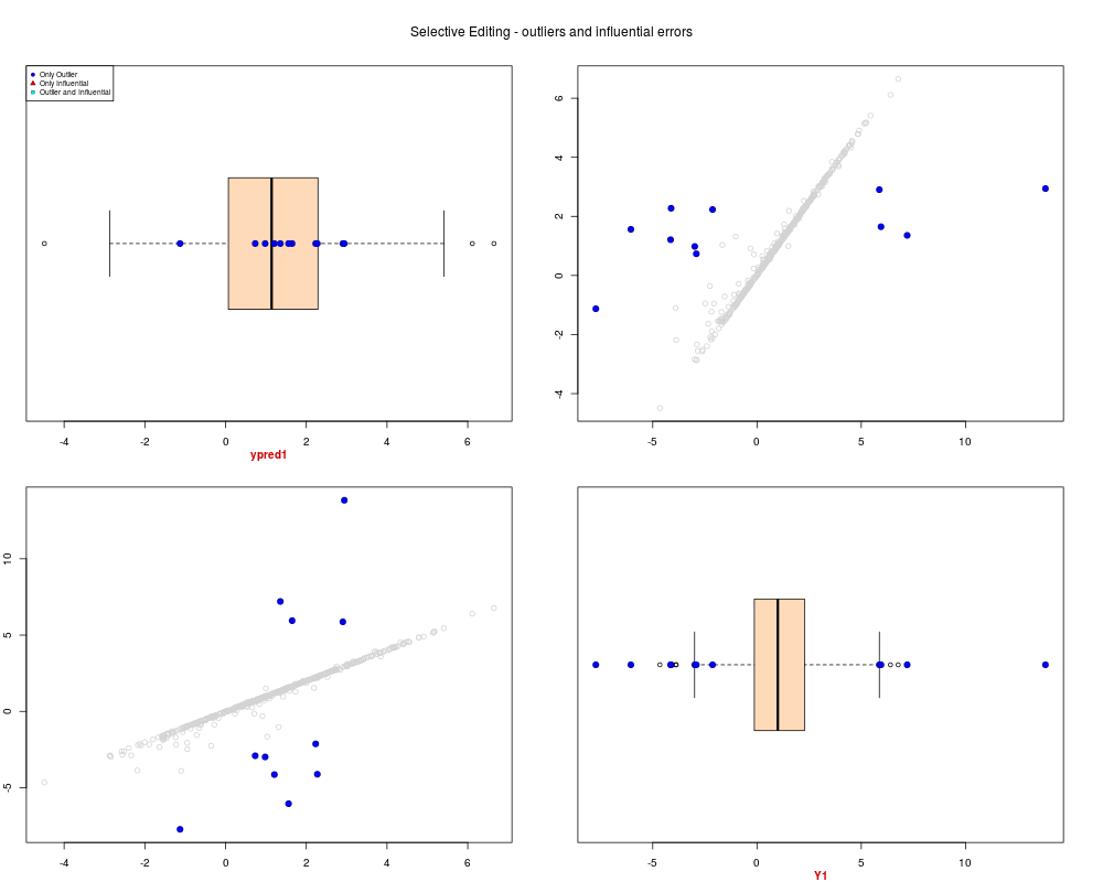
# Plot ypred vs Y1
  sel.pairs(cbind(ypred[,1,drop=FALSE],ex1.data[,"Y1",drop=FALSE]),
            outl=ypred[,"outlier"])

Results

R version 3.3.1 (2016-06-21) -- "Bug in Your Hair"
Copyright (C) 2016 The R Foundation for Statistical Computing
Platform: x86_64-pc-linux-gnu (64-bit)

R is free software and comes with ABSOLUTELY NO WARRANTY.
You are welcome to redistribute it under certain conditions.
Type 'license()' or 'licence()' for distribution details.

R is a collaborative project with many contributors.
Type 'contributors()' for more information and
'citation()' on how to cite R or R packages in publications.

Type 'demo()' for some demos, 'help()' for on-line help, or
'help.start()' for an HTML browser interface to help.
Type 'q()' to quit R.

> library(SeleMix)
Loading required package: mvtnorm
Loading required package: Ecdat
Loading required package: Ecfun

Attaching package: 'Ecfun'

The following object is masked from 'package:base':

    sign


Attaching package: 'Ecdat'

The following object is masked from 'package:datasets':

    Orange

Loading required package: xtable
> png(filename="/home/ddbj/snapshot/RGM3/R_CC/result/SeleMix/pred.y.Rd_%03d_medium.png", width=480, height=480)
> ### Name: pred.y
> ### Title: Prediction of y variables
> ### Aliases: pred.y
> 
> ### ** Examples
> 
> 
> # Parameter estimation with one contaminated variable and one covariate
>   data(ex1.data)
> # Parameters estimated applying ml.est to code{ex1.data} 
>   B1 <- as.matrix(c(-0.152, 1.215))
>   sigma1 <- as.matrix(1.25)
>   lambda1 <- 15.5
>   w1 <- 0.0479
> 
> # Variable prediction
>   ypred <- pred.y (y=ex1.data[,"Y1"],  x=ex1.data[,"X1"], B=B1,
+           sigma=sigma1, lambda=lambda1, w=w1, model="LN", t.outl=0.5)
> # Plot ypred vs Y1
>   sel.pairs(cbind(ypred[,1,drop=FALSE],ex1.data[,"Y1",drop=FALSE]),
+             outl=ypred[,"outlier"])
> 
> 
> 
> 
> 
> dev.off()
null device 
          1 
>