R Graphical Manual

Browse All

Last data update: 2014.03.03

R: Semiparametric regression prediction.

predict.spm

R Documentation

Semiparametric regression prediction.

Description

Takes a fitted spm object produced by spm() and obtains predictions at new data values.

Usage

## S3 method for class 'spm'
predict(object,newdata,se,...)

Arguments

`object`	a fitted `spm` object as produced by `spm()`.
`newdata`	a data frame containing the values of the predictors at which predictions are required. The columns should have the same name as the predictors.
`se`	when this is TRUE standard error estimates are returned for each prediction. The default is FALSE.
`...`	other arguments.

Details

Takes a fitted spm object produced by spm() and obtains predictions at new data values as specified by the ‘newdata’ argument. If ‘se=TRUE’ then standard error estimates are also obtained.

Value

If se=FALSE then a vector of predictions at ‘newdata’ is returned. If se=TRUE then a list with components named ‘fit’ and ‘se’ is returned. The ‘fit’ component contains the predictions. The ‘se’ component contains standard error estimates.

Author(s)

M.P. Wand mwand@uow.edu.au (other contributors listed in SemiPar Users' Manual).

References

Ruppert, D., Wand, M.P. and Carroll, R.J. (2003)
Semiparametric Regression Cambridge University Press.
http://stat.tamu.edu/~carroll/semiregbook/

Ganguli, B. and Wand, M.P. (2005)
SemiPar 1.0 Users' Manual.
http://www.uow.edu.au/~mwand/SPmanu.pdf

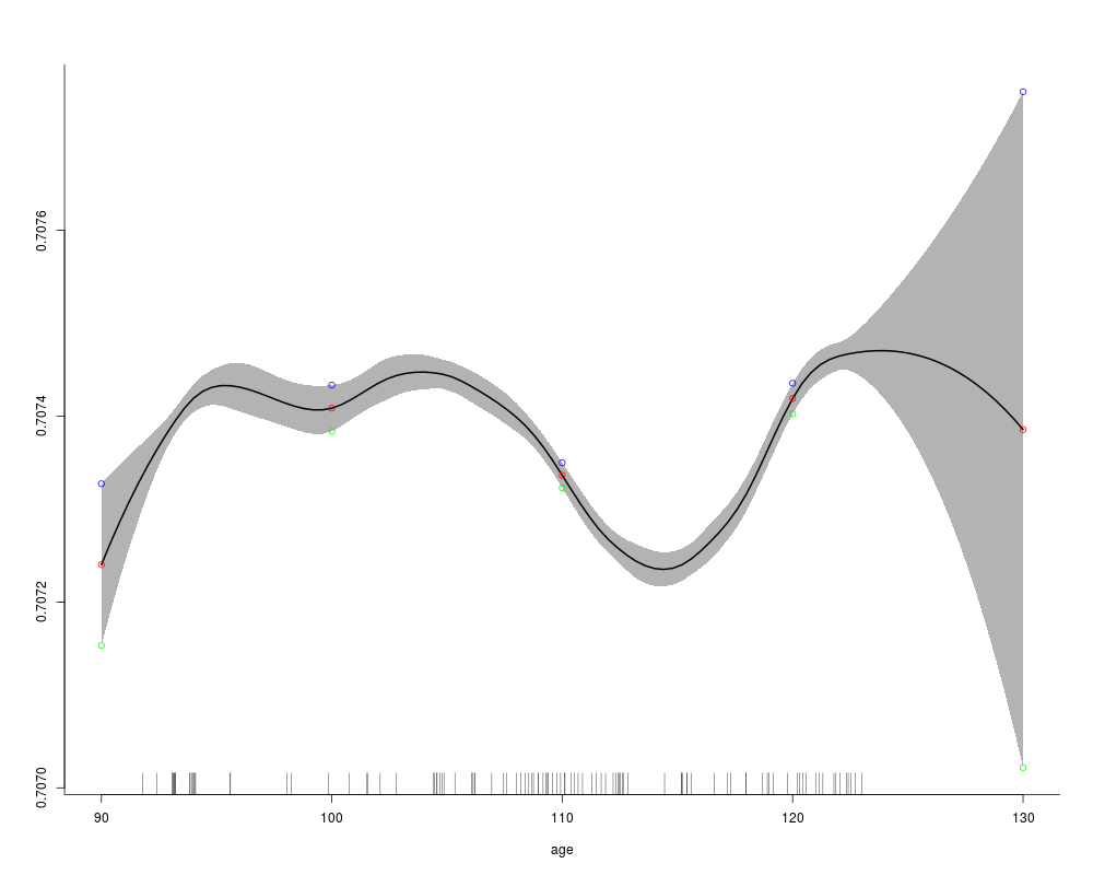
Examples

library(SemiPar)
data(fossil)
attach(fossil)
fit <- spm(strontium.ratio~f(age))
newdata.age <- data.frame(age=c(90,100,110,120,130))
preds <-  predict(fit,newdata=newdata.age,se=TRUE)
print(preds)

plot(fit,xlim=c(90,130))
points(unlist(newdata.age),preds$fit,col="red")
points(unlist(newdata.age),preds$fit+2*preds$se,col="blue")
points(unlist(newdata.age),preds$fit-2*preds$se,col="green")

Results


R version 3.3.1 (2016-06-21) -- "Bug in Your Hair"
Copyright (C) 2016 The R Foundation for Statistical Computing
Platform: x86_64-pc-linux-gnu (64-bit)

R is free software and comes with ABSOLUTELY NO WARRANTY.
You are welcome to redistribute it under certain conditions.
Type 'license()' or 'licence()' for distribution details.

R is a collaborative project with many contributors.
Type 'contributors()' for more information and
'citation()' on how to cite R or R packages in publications.

Type 'demo()' for some demos, 'help()' for on-line help, or
'help.start()' for an HTML browser interface to help.
Type 'q()' to quit R.

> library(SemiPar)
> png(filename="/home/ddbj/snapshot/RGM3/R_CC/result/SemiPar/predict.spm.Rd_%03d_medium.png", width=480, height=480)
> ### Name: predict.spm
> ### Title: Semiparametric regression prediction.
> ### Aliases: predict.spm
> ### Keywords: models smooth regression
> 
> ### ** Examples
> 
> library(SemiPar)
> data(fossil)
> attach(fossil)
> fit <- spm(strontium.ratio~f(age))
> newdata.age <- data.frame(age=c(90,100,110,120,130))
> preds <-  predict(fit,newdata=newdata.age,se=TRUE)
> print(preds)
$fit
[1] 0.7072402 0.7074085 0.7073363 0.7074190 0.7073855

$se
[1] 4.352895e-05 1.241325e-05 6.764932e-06 8.208831e-06 1.818758e-04

> 
> plot(fit,xlim=c(90,130))
> points(unlist(newdata.age),preds$fit,col="red")
> points(unlist(newdata.age),preds$fit+2*preds$se,col="blue")
> points(unlist(newdata.age),preds$fit-2*preds$se,col="green")
> 
> 
> 
> 
> 
> dev.off()
null device 
          1 
>