Semiparametric Copula Bivariate Regression Models

Description

SemiParBIVProbit can be used to fit bivariate binary models where the linear predictors of the two main equations can be flexibly specified using parametric and regression spline components. Several bivariate copula distributions are supported. During the model fitting process, the possible presence of associated error equations, endogeneity, non-random sample selection or partial observability is accounted for. Regression spline bases are extracted from the package mgcv. Multi-dimensional smooths are available via the use of penalized thin plate regression splines. Note that, if it makes sense, the dependence parameter of the employed bivariate distribution can be specified as a function of covariates.

SemiParBIVProbit can also be used to fit bivariate models in which one response is binary and the other is continuous. This case is relevant for estimating, for instance, the effect that a binary endogenous variable has on a continuous response or viceversa or when interest is in modelling jointly binary and continuous responses.

There are many continuous distributions and copula functions that can be employed when using SemiParBIVProbit and we plan to include more options. Other bivariate models can/will be implemented.

Usage

SemiParBIVProbit(formula, data = list(), weights = NULL, subset = NULL,  
                 Model = "B", BivD = "N", 
                 margins = c("probit","probit"), gamlssfit = FALSE,
                 fp = FALSE, hess = TRUE, infl.fac = 1, 
                 rinit = 1, rmax = 100, 
                 iterlimsp = 50, tolsp = 1e-07,
                 gc.l = FALSE, parscale, extra.regI = "t")

Arguments

Details

The bivariate models considered in this package consist of two model equations which depend on flexible linear predictors and whose association between the responses is modelled through parameter θ of a standardised bivariate normal distribution or that of a bivariate copula distribution. The linear predictors of the two equations are flexibly specified using parametric components and smooth functions of covariates. The same can be done for the dependence parameter if it makes sense. Estimation is achieved within a penalized likelihood framework with integrated automatic multiple smoothing parameter selection. The use of penalty matrices allows for the suppression of that part of smooth term complexity which has no support from the data. The trade-off between smoothness and fitness is controlled by smoothing parameters associated with the penalty matrices. Smoothing parameters are chosen to minimise an approximate AIC.

Details of the underlying fitting methods are given in Radice, Marra and Wojtys (in press). Releases previous to 3.2-7 were based on the algorithms detailed in Marra and Radice (2011, 2013).

For sample selection models, if there are factors in the model, before fitting, the user has to ensure that the numbers of factor variables' levels in the selected sample are the same as those in the complete dataset. Even if a model could be fitted in such a situation, the model may produce fits which are not coherent with the nature of the correction sought. As an example consider the situation in which the complete dataset contains a factor variable with five levels and that only three of them appear in the selected sample. For the outcome equation (which is the one of interest) only three levels of such variable exist in the population, but their effects will be corrected for non-random selection using a selection equation in which five levels exist instead. Having differing numbers of factors' levels between complete and selected samples will also make prediction not feasible (an aspect which may be particularly important for selection models); clearly it is not possible to predict the response of interest for the missing entries using a dataset that contains all levels of a factor variable but using an outcome model estimated using a subset of these levels.

Value

The function returns an object of class SemiParBIVProbit as described in SemiParBIVProbitObject.

WARNINGS

Convergence failure may sometimes occur. Convergence can be checked using conv.check which provides some information about the score and information matrix associated with the fitted model. The former should be 0 and the latter positive definite. SemiParBIVProbit() will produce some warnings if there is a convergence issue.

In such a situation, the user may use some extra regularisation (see extra.regI) and/or rescaling (see parscale). Using gamlssfit = TRUE (this is relevant when one outcome is not binary) is typically more effective than the first two options as this will provide better calibrated starting values as compared to those obtained from the default starting value procedure. The default option is, however, gamlssfit = FALSE only because it tends to be computationally cheaper and because the default starting value procedure has typically been found to do a satisfactory job in most cases. (The results obtained when using gamlssfit = FALSE and gamlssfit = TRUE could also be compared to check if starting values make any difference.)

The above suggestions may help, especially the latter option. However, the user should also consider re-specifying the model and/or using a diferrent dependence structure and/or checking that the chosen marginal distribution fit the responses well. In our experience, we found that convergence failure typically occurs when the model has been misspecified and/or the sample size (and/or number of selected observations in selection models) is low compared to the complexity of the model. Examples of misspecification include using a Clayton copula rotated by 90 degrees when a positive association between the margins is present instead, using marginal distributions that do not fit the responses (again, this is a bit more relevant when one of the two responses is continuous), and employing a copula which does not accommodate the type and/or strength of the dependence between the margins (e.g., using AMH when the association between the margins is strong). It is also worth bearing in mind that the use of a three parameter marginal distribution requires the data to be more informative than a situation in which a two parameter distribution is used instead.

When comparing competing models (for instance, by keeping the linear predictor specifications fixed and changing the copula), if the computing time for a set of alternatives is considerably higher than that of another set then it may mean that the more computationally demanding models are not able to fit the data very well (as a higher number of iterations is required to reach convergence). As a practical check, this may be verified by fitting all competing models and, provided convergence is achieved, comparing their respective AIC and BICs, for instance.

In the contexts of endogeneity and non-random sample selection, extra attention is required when specifying the dependence parameter as a function of covariates. This is because in these situations the dependence parameter mainly models the association between the unobserved confounders in the two equations. Therefore, this option would make sense when it is believed that the strength of the association between the unobservables in the two equations varies based on some grouping factor or across geographical areas, for instance.

Author(s)

Maintainer: Giampiero Marra giampiero.marra@ucl.ac.uk

References

Marra G. and Radice R. (2011), Estimation of a Semiparametric Recursive Bivariate Probit in the Presence of Endogeneity. Canadian Journal of Statistics, 39(2), 259-279.

Marra G. and Radice R. (2013), A Penalized Likelihood Estimation Approach to Semiparametric Sample Selection Binary Response Modeling. Electronic Journal of Statistics, 7, 1432-1455.

Marra G., Radice R. and Missiroli S. (2014), Testing the Hypothesis of Absence of Unobserved Confounding in Semiparametric Bivariate Probit Models. Computational Statistics, 29(3-4), 715-741.

Marra G., Radice R. and Filippou P. (in press), Regression Spline Bivariate Probit Models: A Practical Approach to Testing for Exogeneity. Communications in Statistics - Simulation and Computation.

Marra G., Radice R., Barnighausen T., Wood S.N. and McGovern M.E. (submitted). A Simultaneous Equation Approach to Estimating HIV Prevalence with Non-Ignorable Missing Responses.

McGovern M.E., Barnighausen T., Marra G. and Radice R. (2015), On the Assumption of Joint Normality in Selection Models: A Copula Approach Applied to Estimating HIV Prevalence. Epidemiology, 26(2), 229-237.

Radice R., Marra G. and M. Wojtys (in press), Copula Regression Spline Models for Binary Outcomes. Statistics and Computing.

Marra G. and Wood S.N. (2011), Practical Variable Selection for Generalized Additive Models. Computational Statistics and Data Analysis, 55(7), 2372-2387.

Marra G. and Wood S.N. (2012), Coverage Properties of Confidence Intervals for Generalized Additive Model Components. Scandinavian Journal of Statistics, 39(1), 53-74.

Poirier D.J. (1980), Partial Observability in Bivariate Probit Models. Journal of Econometrics, 12, 209-217.

Wood S.N. (2004), Stable and efficient multiple smoothing parameter estimation for generalized additive models. Journal of the American Statistical Association, 99(467), 673-686.

See Also

copulaReg, copulaSampleSel, AT, OR, RR, adjCov, prev, gt.bpm, LM.bpm, VuongClarke, plot.SemiParBIVProbit, SemiParBIVProbit-package, SemiParBIVProbitObject, conv.check, summary.SemiParBIVProbit, predict.SemiParBIVProbit

Examples

library(SemiParBIVProbit)

############
## EXAMPLE 1
############
## Generate data
## Correlation between the two equations 0.5 - Sample size 400 

set.seed(0)

n <- 400

Sigma <- matrix(0.5, 2, 2); diag(Sigma) <- 1
u     <- rMVN(n, rep(0,2), Sigma)

x1 <- round(runif(n)); x2 <- runif(n); x3 <- runif(n)

f1   <- function(x) cos(pi*2*x) + sin(pi*x)
f2   <- function(x) x+exp(-30*(x-0.5)^2)   

y1 <- ifelse(-1.55 + 2*x1    + f1(x2) + u[,1] > 0, 1, 0)
y2 <- ifelse(-0.25 - 1.25*x1 + f2(x2) + u[,2] > 0, 1, 0)

dataSim <- data.frame(y1, y2, x1, x2, x3)

#
#

## CLASSIC BIVARIATE PROBIT

out  <- SemiParBIVProbit(list(y1 ~ x1 + x2 + x3, 
                              y2 ~ x1 + x2 + x3), 
                         data = dataSim)
conv.check(out)
summary(out)
AIC(out)
BIC(out)

## SEMIPARAMETRIC BIVARIATE PROBIT

## "cr" cubic regression spline basis      - "cs" shrinkage version of "cr"
## "tp" thin plate regression spline basis - "ts" shrinkage version of "tp"
## for smooths of one variable, "cr/cs" and "tp/ts" achieve similar results 
## k is the basis dimension - default is 10
## m is the order of the penalty for the specific term - default is 2
## For COPULA models use BivD argument 

out  <- SemiParBIVProbit(list(y1 ~ x1 + s(x2, bs = "tp", k = 10, m = 2) + s(x3), 
                              y2 ~ x1 + s(x2) + s(x3)),  
                         data = dataSim)
conv.check(out)
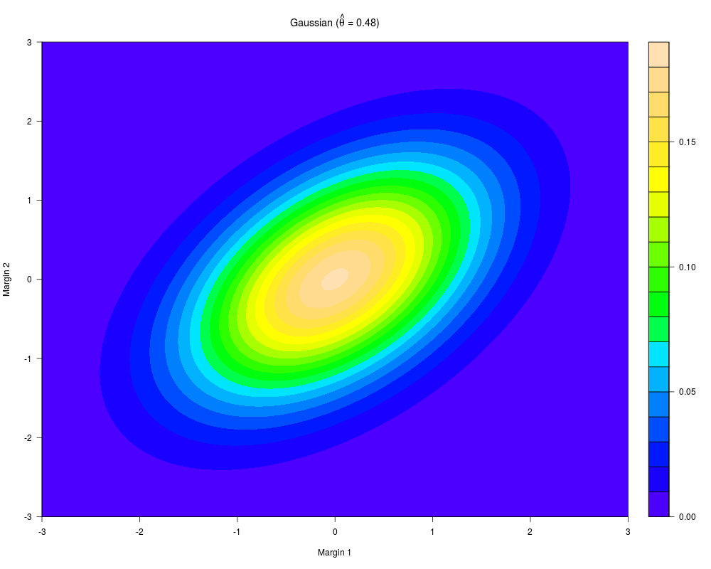
summary(out, cm.plot = TRUE)
AIC(out)


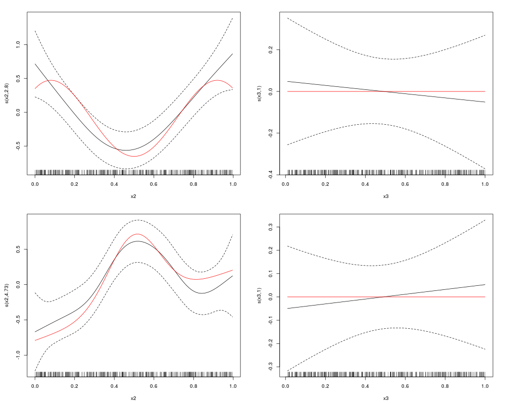
## estimated smooth function plots - red lines are true curves

x2 <- sort(x2)
f1.x2 <- f1(x2)[order(x2)] - mean(f1(x2))
f2.x2 <- f2(x2)[order(x2)] - mean(f2(x2))
f3.x3 <- rep(0, length(x3))

par(mfrow=c(2,2),mar=c(4.5,4.5,2,2))
plot(out, eq = 1, select = 1, seWithMean = TRUE, scale = 0)
lines(x2, f1.x2, col = "red")
plot(out, eq = 1, select = 2, seWithMean = TRUE, scale = 0)
lines(x3, f3.x3, col = "red")
plot(out, eq = 2, select = 1, seWithMean = TRUE, scale = 0)
lines(x2, f2.x2, col = "red")
plot(out, eq = 2, select = 2, seWithMean = TRUE, scale = 0)
lines(x3, f3.x3, col = "red")

## p-values suggest to drop x3 from both equations, with a stronger 
## evidence for eq. 2. This can be also achieved using shrinkage smoothers

outSS <- SemiParBIVProbit(list(y1 ~ x1 + s(x2, bs = "ts") + s(x3, bs = "cs"), 
                               y2 ~ x1 + s(x2, bs = "cs") + s(x3, bs = "ts")), 
                          data = dataSim)
conv.check(outSS)                          

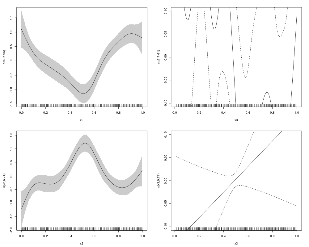
plot(outSS, eq = 1, select = 1, scale = 0, shade = TRUE)
plot(outSS, eq = 1, select = 2, ylim = c(-0.1,0.1))
plot(outSS, eq = 2, select = 1, scale = 0, shade = TRUE)
plot(outSS, eq = 2, select = 2, ylim = c(-0.1,0.1))

## Not run:  

## SEMIPARAMETRIC BIVARIATE PROBIT with association parameter 
## depending on covariates as well

eq.mu.1  <- y1 ~ x1 + s(x2)
eq.mu.2  <- y2 ~ x1 + s(x2)
eq.theta <-    ~ x1 + s(x2)

fl <- list(eq.mu.1, eq.mu.2, eq.theta)

outD <- SemiParBIVProbit(fl, data = dataSim)
conv.check(outD)  
summary(outD)
outD$theta

plot(outD, eq = 1, seWithMean = TRUE)
plot(outD, eq = 2, seWithMean = TRUE)
plot(outD, eq = 3, seWithMean = TRUE)
graphics.off()

#
#

############
## EXAMPLE 2
############
## Generate data with one endogenous variable 
## and exclusion restriction

set.seed(0)

n <- 400

Sigma <- matrix(0.5, 2, 2); diag(Sigma) <- 1
u     <- rMVN(n, rep(0,2), Sigma)

cov   <- rMVN(n, rep(0,2), Sigma)
cov   <- pnorm(cov)
x1 <- round(cov[,1]); x2 <- cov[,2]

f1   <- function(x) cos(pi*2*x) + sin(pi*x)
f2   <- function(x) x+exp(-30*(x-0.5)^2)   

y1 <- ifelse(-1.55 + 2*x1    + f1(x2) + u[,1] > 0, 1, 0)
y2 <- ifelse(-0.25 - 1.25*y1 + f2(x2) + u[,2] > 0, 1, 0)

dataSim <- data.frame(y1, y2, x1, x2)

#

## Testing the hypothesis of absence of endogeneity... 

LM.bpm(list(y1 ~ x1 + s(x2), y2 ~ y1 + s(x2)), dataSim, Model = "B")

# p-value suggests presence of endogeneity, hence fit a bivariate model


## CLASSIC RECURSIVE BIVARIATE PROBIT

out <- SemiParBIVProbit(list(y1 ~ x1 + x2, 
                             y2 ~ y1 + x2), 
                        data = dataSim)
conv.check(out)                        
summary(out)
AIC(out); BIC(out)

## SEMIPARAMETRIC RECURSIVE BIVARIATE PROBIT

out <- SemiParBIVProbit(list(y1 ~ x1 + s(x2), 
                             y2 ~ y1 + s(x2)), 
                        data = dataSim)
conv.check(out)                        
summary(out)
AIC(out); BIC(out)

#

## Testing the hypothesis of absence of endogeneity post estimation... 

gt.bpm(out)

#
## reatment effect, risk ratio and odds ratio with CIs

mb(y1, y2, Model = "B")
AT(out, nm.end = "y1", hd.plot = TRUE) 
RR(out, nm.end = "y1") 
OR(out, nm.end = "y1") 
AT(out, nm.end = "y1", type = "univariate") 


## try a Clayton copula model... 

outC <- SemiParBIVProbit(list(y1 ~ x1 + s(x2), 
                              y2 ~ y1 + s(x2)), 
                         data = dataSim, BivD = "C0")
conv.check(outC)                         
summary(outC)
AT(outC, nm.end = "y1") 

## try a Joe copula model... 

outJ <- SemiParBIVProbit(list(y1 ~ x1 + s(x2), 
                              y2 ~ y1 + s(x2)), 
                         data = dataSim, BivD = "J0")
conv.check(outJ)
summary(outJ, cm.plot = TRUE)
AT(outJ, "y1") 


VuongClarke(out, outJ)

#
## recursive bivariate probit modelling with unpenalized splines 
## can be achieved as follows

outFP <- SemiParBIVProbit(list(y1 ~ x1 + s(x2, bs = "cr", k = 5), 
                               y2 ~ y1 + s(x2, bs = "cr", k = 6)), 
                          fp = TRUE, data = dataSim)
conv.check(outFP)                            
summary(outFP)

# in the above examples a third equation could be introduced
# as illustrated in Example 1

#
#################
## See also ?meps
#################

############
## EXAMPLE 3
############
## Generate data with a non-random sample selection mechanism 
## and exclusion restriction

set.seed(0)

n <- 2000

Sigma <- matrix(0.5, 2, 2); diag(Sigma) <- 1
u     <- rMVN(n, rep(0,2), Sigma)

SigmaC <- matrix(0.5, 3, 3); diag(SigmaC) <- 1
cov    <- rMVN(n, rep(0,3), SigmaC)
cov    <- pnorm(cov)
bi <- round(cov[,1]); x1 <- cov[,2]; x2 <- cov[,3]
  
f11 <- function(x) -0.7*(4*x + 2.5*x^2 + 0.7*sin(5*x) + cos(7.5*x))
f12 <- function(x) -0.4*( -0.3 - 1.6*x + sin(5*x))  
f21 <- function(x) 0.6*(exp(x) + sin(2.9*x)) 

ys <-  0.58 + 2.5*bi + f11(x1) + f12(x2) + u[, 1] > 0
y  <- -0.68 - 1.5*bi + f21(x1) +         + u[, 2] > 0
yo <- y*(ys > 0)
  
dataSim <- data.frame(y, ys, yo, bi, x1, x2)

## Testing the hypothesis of absence of non-random sample selection... 

LM.bpm(list(ys ~ bi + s(x1) + s(x2), yo ~ bi + s(x1)), dataSim, Model = "BSS")

# p-value suggests presence of sample selection, hence fit a bivariate model

#
## SEMIPARAMETRIC SAMPLE SELECTION BIVARIATE PROBIT
## the first equation MUST be the selection equation

out <- SemiParBIVProbit(list(ys ~ bi + s(x1) + s(x2), 
                             yo ~ bi + s(x1)), 
                        data = dataSim, Model = "BSS")
conv.check(out)                          
gt.bpm(out)                        

## compare the two summary outputs
## the second output produces a summary of the results obtained when
## selection bias is not accounted for

summary(out)
summary(out$gam2)

## corrected predicted probability that 'yo' is equal to 1

mb(ys, yo, Model = "BSS")
prev(out, hd.plot = TRUE)
prev(out, type = "univariate", hd.plot = TRUE)

## estimated smooth function plots
## the red line is the true curve
## the blue line is the univariate model curve not accounting for selection bias

x1.s <- sort(x1[dataSim$ys>0])
f21.x1 <- f21(x1.s)[order(x1.s)]-mean(f21(x1.s))

plot(out, eq = 2, ylim = c(-1.65,0.95)); lines(x1.s, f21.x1, col="red")
par(new = TRUE)
plot(out$gam2, se = FALSE, col = "blue", ylim = c(-1.65,0.95), 
     ylab = "", rug = FALSE)

#
#
## try a Clayton copula model... 

outC <- SemiParBIVProbit(list(ys ~ bi + s(x1) + s(x2), 
                              yo ~ bi + s(x1)), 
                         data = dataSim, Model = "BSS", BivD = "C0")
conv.check(outC)
summary(outC, cm.plot = TRUE)
prev(outC)

# in the above examples a third equation could be introduced
# as illustrated in Example 1

#
################
## See also ?hiv
################

############
## EXAMPLE 4
############
## Generate data with partial observability

set.seed(0)

n <- 10000

Sigma <- matrix(0.5, 2, 2); diag(Sigma) <- 1
u     <- rMVN(n, rep(0,2), Sigma)

x1 <- round(runif(n)); x2 <- runif(n); x3 <- runif(n)

y1 <- ifelse(-1.55 + 2*x1 + x2 + u[,1] > 0, 1, 0)
y2 <- ifelse( 0.45 - x3        + u[,2] > 0, 1, 0)
y  <- y1*y2

dataSim <- data.frame(y, x1, x2, x3)


## BIVARIATE PROBIT with Partial Observability

out  <- SemiParBIVProbit(list(y ~ x1 + x2, 
                              y ~ x3), 
                         data = dataSim, Model = "BPO")
conv.check(out)
summary(out)

# first ten estimated probabilities for the four events from object out

cbind(out$p11, out$p10, out$p00, out$p01)[1:10,]


# case with smooth function 
# (more computationally intensive)  

f1 <- function(x) cos(pi*2*x) + sin(pi*x)

y1 <- ifelse(-1.55 + 2*x1 + f1(x2) + u[,1] > 0, 1, 0)
y2 <- ifelse( 0.45 - x3            + u[,2] > 0, 1, 0)
y  <- y1*y2

dataSim <- data.frame(y, x1, x2, x3)

out  <- SemiParBIVProbit(list(y ~ x1 + s(x2), 
                              y ~ x3), 
                         data = dataSim, Model = "BPO")

conv.check(out)
summary(out, cm.plot = TRUE)


# plot estimated and true functions

x2 <- sort(x2); f1.x2 <- f1(x2)[order(x2)] - mean(f1(x2))
plot(out, eq = 1, scale = 0); lines(x2, f1.x2, col = "red")

#
################
## See also ?war
################

############
## EXAMPLE 5
############
## Generate data with one endogenous binary variable 
## and continuous outcome

set.seed(0)

n <- 1000

Sigma <- matrix(0.5, 2, 2); diag(Sigma) <- 1
u     <- rMVN(n, rep(0,2), Sigma)

cov   <- rMVN(n, rep(0,2), Sigma)
cov   <- pnorm(cov)
x1 <- round(cov[,1]); x2 <- cov[,2]

f1   <- function(x) cos(pi*2*x) + sin(pi*x)
f2   <- function(x) x+exp(-30*(x-0.5)^2)   

y1 <- ifelse(-1.55 + 2*x1    + f1(x2) + u[,1] > 0, 1, 0)
y2 <-        -0.25 - 1.25*y1 + f2(x2) + u[,2] 

dataSim <- data.frame(y1, y2, x1, x2)


## RECURSIVE Model

rc <- resp.check(y2, margin = "N", print.par = TRUE, loglik = TRUE)
AIC(rc); BIC(rc)

out <- SemiParBIVProbit(list(y1 ~ x1 + x2, 
                             y2 ~ y1 + x2), 
                        data = dataSim, margins = c("probit","N"))
conv.check(out)                        
summary(out)
post.check(out)

## SEMIPARAMETRIC RECURSIVE Model

eq.mu.1   <- y1 ~ x1 + s(x2) 
eq.mu.2   <- y2 ~ y1 + s(x2)
eq.sigma2 <-    ~ 1
eq.theta  <-    ~ 1

fl <- list(eq.mu.1, eq.mu.2, eq.sigma2, eq.theta)

out <- SemiParBIVProbit(fl, data = dataSim, 
                        margins = c("probit","N"), gamlssfit = TRUE)
conv.check(out)                        
summary(out)
post.check(out)
jc.probs(out, 1, 1.5, intervals = TRUE)[1:4,]
AT(out, nm.end = "y1")
AT(out, nm.end = "y1", type = "univariate")


#
#

############
## EXAMPLE 6
############
## Generate data with one endogenous continuous exposure 
## and binary outcome

set.seed(0)

n <- 1000

Sigma <- matrix(0.5, 2, 2); diag(Sigma) <- 1
u     <- rMVN(n, rep(0,2), Sigma)

cov   <- rMVN(n, rep(0,2), Sigma)
cov   <- pnorm(cov)
x1 <- round(cov[,1]); x2 <- cov[,2]

f1   <- function(x) cos(pi*2*x) + sin(pi*x)
f2   <- function(x) x+exp(-30*(x-0.5)^2) 

y1 <-        -0.25 - 2*x1    + f2(x2) + u[,2] 
y2 <- ifelse(-0.25 - 0.25*y1 + f1(x2) + u[,1] > 0, 1, 0)

dataSim <- data.frame(y1, y2, x1, x2)

eq.mu.1   <- y2 ~ y1 + s(x2) 
eq.mu.2   <- y1 ~ x1 + s(x2)
eq.sigma2 <-    ~ 1
eq.theta  <-    ~ 1

fl <- list(eq.mu.1, eq.mu.2, eq.sigma2, eq.theta)

out <- SemiParBIVProbit(fl, data = dataSim, 
                        margins = c("probit","N"))
conv.check(out)                        
summary(out)
post.check(out)
AT(out, nm.end = "y1")
AT(out, nm.end = "y1", type = "univariate")
RR(out, nm.end = "y1", rr.plot = TRUE)
RR(out, nm.end = "y1", type = "univariate")
OR(out, nm.end = "y1", or.plot = TRUE)
OR(out, nm.end = "y1", type = "univariate")


## End(Not run)

Results

R version 3.3.1 (2016-06-21) -- "Bug in Your Hair"
Copyright (C) 2016 The R Foundation for Statistical Computing
Platform: x86_64-pc-linux-gnu (64-bit)

R is free software and comes with ABSOLUTELY NO WARRANTY.
You are welcome to redistribute it under certain conditions.
Type 'license()' or 'licence()' for distribution details.

R is a collaborative project with many contributors.
Type 'contributors()' for more information and
'citation()' on how to cite R or R packages in publications.

Type 'demo()' for some demos, 'help()' for on-line help, or
'help.start()' for an HTML browser interface to help.
Type 'q()' to quit R.

> library(SemiParBIVProbit)
Loading required package: mgcv
Loading required package: nlme
This is mgcv 1.8-12. For overview type 'help("mgcv-package")'.

This is SemiParBIVProbit 3.7-1.
For overview type 'help("SemiParBIVProbit-package")'.

> png(filename="/home/ddbj/snapshot/RGM3/R_CC/result/SemiParBIVProbit/SemiParBIVProbit.Rd_%03d_medium.png", width=480, height=480)
> ### Name: SemiParBIVProbit
> ### Title: Semiparametric Copula Bivariate Regression Models
> ### Aliases: SemiParBIVProbit
> ### Keywords: non-random sample selection semiparametric bivariate
> ###   modelling partial observability endogeneity smooth regression spline
> ###   shrinkage smoother variable selection
> 
> ### ** Examples
> 
> 
> library(SemiParBIVProbit)
> 
> ############
> ## EXAMPLE 1
> ############
> ## Generate data
> ## Correlation between the two equations 0.5 - Sample size 400 
> 
> set.seed(0)
> 
> n <- 400
> 
> Sigma <- matrix(0.5, 2, 2); diag(Sigma) <- 1
> u     <- rMVN(n, rep(0,2), Sigma)
> 
> x1 <- round(runif(n)); x2 <- runif(n); x3 <- runif(n)
> 
> f1   <- function(x) cos(pi*2*x) + sin(pi*x)
> f2   <- function(x) x+exp(-30*(x-0.5)^2)   
> 
> y1 <- ifelse(-1.55 + 2*x1    + f1(x2) + u[,1] > 0, 1, 0)
> y2 <- ifelse(-0.25 - 1.25*x1 + f2(x2) + u[,2] > 0, 1, 0)
> 
> dataSim <- data.frame(y1, y2, x1, x2, x3)
> 
> #
> #
> 
> ## CLASSIC BIVARIATE PROBIT
> 
> out  <- SemiParBIVProbit(list(y1 ~ x1 + x2 + x3, 
+                               y2 ~ x1 + x2 + x3), 
+                          data = dataSim)
> conv.check(out)

Largest absolute gradient value: 9.321016e-14
Observed information matrix is positive definite
Eigenvalue range: [9.528687,419.9106]

Trust region iterations: 3 

> summary(out)

COPULA:   Gaussian
MARGIN 1: Bernoulli
MARGIN 2: Bernoulli

EQUATION 1
Link function for mu.1: probit 
Formula: y1 ~ x1 + x2 + x3

Parametric coefficients:
            Estimate Std. Error z value Pr(>|z|)    
(Intercept) -0.94936    0.20532  -4.624 3.77e-06 ***
x1           1.97383    0.15150  13.028  < 2e-16 ***
x2           0.20574    0.25474   0.808    0.419    
x3          -0.06393    0.25939  -0.246    0.805    
---
Signif. codes:  0 '***' 0.001 '**' 0.01 '*' 0.05 '.' 0.1 ' ' 1


EQUATION 2
Link function for mu.2: probit 
Formula: y2 ~ x1 + x2 + x3

Parametric coefficients:
            Estimate Std. Error z value Pr(>|z|)    
(Intercept)  0.04474    0.17736   0.252  0.80084    
x1          -1.07918    0.13393  -8.058 7.76e-16 ***
x2           0.66869    0.23016   2.905  0.00367 ** 
x3           0.08599    0.23228   0.370  0.71124    
---
Signif. codes:  0 '***' 0.001 '**' 0.01 '*' 0.05 '.' 0.1 ' ' 1


n = 400  theta = 0.282(0.062,0.458)  tau = 0.182(0.0395,0.303)
total edf = 9

> AIC(out)
[1] 840.3036
> BIC(out)
[1] 876.2268
> 
> ## SEMIPARAMETRIC BIVARIATE PROBIT
> 
> ## "cr" cubic regression spline basis      - "cs" shrinkage version of "cr"
> ## "tp" thin plate regression spline basis - "ts" shrinkage version of "tp"
> ## for smooths of one variable, "cr/cs" and "tp/ts" achieve similar results 
> ## k is the basis dimension - default is 10
> ## m is the order of the penalty for the specific term - default is 2
> ## For COPULA models use BivD argument 
> 
> out  <- SemiParBIVProbit(list(y1 ~ x1 + s(x2, bs = "tp", k = 10, m = 2) + s(x3), 
+                               y2 ~ x1 + s(x2) + s(x3)),  
+                          data = dataSim)
> conv.check(out)

Largest absolute gradient value: 1.485398e-09
Observed information matrix is positive definite
Eigenvalue range: [0.2372136,5.216988e+13]

Trust region iterations before smoothing parameter estimation: 4
Loops for smoothing parameter estimation: 3
Trust region iterations within smoothing loops: 4 

> summary(out, cm.plot = TRUE)

COPULA:   Gaussian
MARGIN 1: Bernoulli
MARGIN 2: Bernoulli

EQUATION 1
Link function for mu.1: probit 
Formula: y1 ~ x1 + s(x2, bs = "tp", k = 10, m = 2) + s(x3)

Parametric coefficients:
            Estimate Std. Error z value Pr(>|z|)    
(Intercept)  -0.9852     0.1094  -9.005   <2e-16 ***
x1            2.1885     0.1691  12.940   <2e-16 ***
---
Signif. codes:  0 '***' 0.001 '**' 0.01 '*' 0.05 '.' 0.1 ' ' 1

Smooth components' approximate significance:
        edf Ref.df Chi.sq  p-value    
s(x2) 2.805  3.499 31.721 1.87e-06 ***
s(x3) 1.000  1.000  0.134    0.714    
---
Signif. codes:  0 '***' 0.001 '**' 0.01 '*' 0.05 '.' 0.1 ' ' 1


EQUATION 2
Link function for mu.2: probit 
Formula: y2 ~ x1 + s(x2) + s(x3)

Parametric coefficients:
            Estimate Std. Error z value Pr(>|z|)    
(Intercept)  0.43374    0.09316   4.656 3.22e-06 ***
x1          -1.14477    0.13880  -8.248  < 2e-16 ***
---
Signif. codes:  0 '***' 0.001 '**' 0.01 '*' 0.05 '.' 0.1 ' ' 1

Smooth components' approximate significance:
        edf Ref.df Chi.sq  p-value    
s(x2) 4.728  5.784 33.810 6.81e-06 ***
s(x3) 1.000  1.000  0.189    0.664    
---
Signif. codes:  0 '***' 0.001 '**' 0.01 '*' 0.05 '.' 0.1 ' ' 1


n = 400  theta = 0.484(0.324,0.646)  tau = 0.322(0.21,0.447)
total edf = 14.5

> AIC(out)
[1] 774.3511
> 
> 
> ## estimated smooth function plots - red lines are true curves
> 
> x2 <- sort(x2)
> f1.x2 <- f1(x2)[order(x2)] - mean(f1(x2))
> f2.x2 <- f2(x2)[order(x2)] - mean(f2(x2))
> f3.x3 <- rep(0, length(x3))
> 
> par(mfrow=c(2,2),mar=c(4.5,4.5,2,2))
> plot(out, eq = 1, select = 1, seWithMean = TRUE, scale = 0)
> lines(x2, f1.x2, col = "red")
> plot(out, eq = 1, select = 2, seWithMean = TRUE, scale = 0)
> lines(x3, f3.x3, col = "red")
> plot(out, eq = 2, select = 1, seWithMean = TRUE, scale = 0)
> lines(x2, f2.x2, col = "red")
> plot(out, eq = 2, select = 2, seWithMean = TRUE, scale = 0)
> lines(x3, f3.x3, col = "red")
> 
> ## p-values suggest to drop x3 from both equations, with a stronger 
> ## evidence for eq. 2. This can be also achieved using shrinkage smoothers
> 
> outSS <- SemiParBIVProbit(list(y1 ~ x1 + s(x2, bs = "ts") + s(x3, bs = "cs"), 
+                                y2 ~ x1 + s(x2, bs = "cs") + s(x3, bs = "ts")), 
+                           data = dataSim)
Warning message:
Largest absolute gradient value is not close to 0. 
 Read the WARNINGS section in ?SemiParBIVProbit. 
> conv.check(outSS)                          

Largest absolute gradient value: 1.747239
Observed information matrix is positive definite
Eigenvalue range: [5.711081e-129,449317]

Trust region iterations before smoothing parameter estimation: 4
Loops for smoothing parameter estimation: 4
Trust region iterations within smoothing loops: 174 

> 
> plot(outSS, eq = 1, select = 1, scale = 0, shade = TRUE)
> plot(outSS, eq = 1, select = 2, ylim = c(-0.1,0.1))
> plot(outSS, eq = 2, select = 1, scale = 0, shade = TRUE)
> plot(outSS, eq = 2, select = 2, ylim = c(-0.1,0.1))
> 
> ## Not run: 
> ##D  
> ##D 
> ##D ## SEMIPARAMETRIC BIVARIATE PROBIT with association parameter 
> ##D ## depending on covariates as well
> ##D 
> ##D eq.mu.1  <- y1 ~ x1 + s(x2)
> ##D eq.mu.2  <- y2 ~ x1 + s(x2)
> ##D eq.theta <-    ~ x1 + s(x2)
> ##D 
> ##D fl <- list(eq.mu.1, eq.mu.2, eq.theta)
> ##D 
> ##D outD <- SemiParBIVProbit(fl, data = dataSim)
> ##D conv.check(outD)  
> ##D summary(outD)
> ##D outD$theta
> ##D 
> ##D plot(outD, eq = 1, seWithMean = TRUE)
> ##D plot(outD, eq = 2, seWithMean = TRUE)
> ##D plot(outD, eq = 3, seWithMean = TRUE)
> ##D graphics.off()
> ##D 
> ##D #
> ##D #
> ##D 
> ##D ############
> ##D ## EXAMPLE 2
> ##D ############
> ##D ## Generate data with one endogenous variable 
> ##D ## and exclusion restriction
> ##D 
> ##D set.seed(0)
> ##D 
> ##D n <- 400
> ##D 
> ##D Sigma <- matrix(0.5, 2, 2); diag(Sigma) <- 1
> ##D u     <- rMVN(n, rep(0,2), Sigma)
> ##D 
> ##D cov   <- rMVN(n, rep(0,2), Sigma)
> ##D cov   <- pnorm(cov)
> ##D x1 <- round(cov[,1]); x2 <- cov[,2]
> ##D 
> ##D f1   <- function(x) cos(pi*2*x) + sin(pi*x)
> ##D f2   <- function(x) x+exp(-30*(x-0.5)^2)   
> ##D 
> ##D y1 <- ifelse(-1.55 + 2*x1    + f1(x2) + u[,1] > 0, 1, 0)
> ##D y2 <- ifelse(-0.25 - 1.25*y1 + f2(x2) + u[,2] > 0, 1, 0)
> ##D 
> ##D dataSim <- data.frame(y1, y2, x1, x2)
> ##D 
> ##D #
> ##D 
> ##D ## Testing the hypothesis of absence of endogeneity... 
> ##D 
> ##D LM.bpm(list(y1 ~ x1 + s(x2), y2 ~ y1 + s(x2)), dataSim, Model = "B")
> ##D 
> ##D # p-value suggests presence of endogeneity, hence fit a bivariate model
> ##D 
> ##D 
> ##D ## CLASSIC RECURSIVE BIVARIATE PROBIT
> ##D 
> ##D out <- SemiParBIVProbit(list(y1 ~ x1 + x2, 
> ##D                              y2 ~ y1 + x2), 
> ##D                         data = dataSim)
> ##D conv.check(out)                        
> ##D summary(out)
> ##D AIC(out); BIC(out)
> ##D 
> ##D ## SEMIPARAMETRIC RECURSIVE BIVARIATE PROBIT
> ##D 
> ##D out <- SemiParBIVProbit(list(y1 ~ x1 + s(x2), 
> ##D                              y2 ~ y1 + s(x2)), 
> ##D                         data = dataSim)
> ##D conv.check(out)                        
> ##D summary(out)
> ##D AIC(out); BIC(out)
> ##D 
> ##D #
> ##D 
> ##D ## Testing the hypothesis of absence of endogeneity post estimation... 
> ##D 
> ##D gt.bpm(out)
> ##D 
> ##D #
> ##D ## reatment effect, risk ratio and odds ratio with CIs
> ##D 
> ##D mb(y1, y2, Model = "B")
> ##D AT(out, nm.end = "y1", hd.plot = TRUE) 
> ##D RR(out, nm.end = "y1") 
> ##D OR(out, nm.end = "y1") 
> ##D AT(out, nm.end = "y1", type = "univariate") 
> ##D 
> ##D 
> ##D ## try a Clayton copula model... 
> ##D 
> ##D outC <- SemiParBIVProbit(list(y1 ~ x1 + s(x2), 
> ##D                               y2 ~ y1 + s(x2)), 
> ##D                          data = dataSim, BivD = "C0")
> ##D conv.check(outC)                         
> ##D summary(outC)
> ##D AT(outC, nm.end = "y1") 
> ##D 
> ##D ## try a Joe copula model... 
> ##D 
> ##D outJ <- SemiParBIVProbit(list(y1 ~ x1 + s(x2), 
> ##D                               y2 ~ y1 + s(x2)), 
> ##D                          data = dataSim, BivD = "J0")
> ##D conv.check(outJ)
> ##D summary(outJ, cm.plot = TRUE)
> ##D AT(outJ, "y1") 
> ##D 
> ##D 
> ##D VuongClarke(out, outJ)
> ##D 
> ##D #
> ##D ## recursive bivariate probit modelling with unpenalized splines 
> ##D ## can be achieved as follows
> ##D 
> ##D outFP <- SemiParBIVProbit(list(y1 ~ x1 + s(x2, bs = "cr", k = 5), 
> ##D                                y2 ~ y1 + s(x2, bs = "cr", k = 6)), 
> ##D                           fp = TRUE, data = dataSim)
> ##D conv.check(outFP)                            
> ##D summary(outFP)
> ##D 
> ##D # in the above examples a third equation could be introduced
> ##D # as illustrated in Example 1
> ##D 
> ##D #
> ##D #################
> ##D ## See also ?meps
> ##D #################
> ##D 
> ##D ############
> ##D ## EXAMPLE 3
> ##D ############
> ##D ## Generate data with a non-random sample selection mechanism 
> ##D ## and exclusion restriction
> ##D 
> ##D set.seed(0)
> ##D 
> ##D n <- 2000
> ##D 
> ##D Sigma <- matrix(0.5, 2, 2); diag(Sigma) <- 1
> ##D u     <- rMVN(n, rep(0,2), Sigma)
> ##D 
> ##D SigmaC <- matrix(0.5, 3, 3); diag(SigmaC) <- 1
> ##D cov    <- rMVN(n, rep(0,3), SigmaC)
> ##D cov    <- pnorm(cov)
> ##D bi <- round(cov[,1]); x1 <- cov[,2]; x2 <- cov[,3]
> ##D   
> ##D f11 <- function(x) -0.7*(4*x + 2.5*x^2 + 0.7*sin(5*x) + cos(7.5*x))
> ##D f12 <- function(x) -0.4*( -0.3 - 1.6*x + sin(5*x))  
> ##D f21 <- function(x) 0.6*(exp(x) + sin(2.9*x)) 
> ##D 
> ##D ys <-  0.58 + 2.5*bi + f11(x1) + f12(x2) + u[, 1] > 0
> ##D y  <- -0.68 - 1.5*bi + f21(x1) +         + u[, 2] > 0
> ##D yo <- y*(ys > 0)
> ##D   
> ##D dataSim <- data.frame(y, ys, yo, bi, x1, x2)
> ##D 
> ##D ## Testing the hypothesis of absence of non-random sample selection... 
> ##D 
> ##D LM.bpm(list(ys ~ bi + s(x1) + s(x2), yo ~ bi + s(x1)), dataSim, Model = "BSS")
> ##D 
> ##D # p-value suggests presence of sample selection, hence fit a bivariate model
> ##D 
> ##D #
> ##D ## SEMIPARAMETRIC SAMPLE SELECTION BIVARIATE PROBIT
> ##D ## the first equation MUST be the selection equation
> ##D 
> ##D out <- SemiParBIVProbit(list(ys ~ bi + s(x1) + s(x2), 
> ##D                              yo ~ bi + s(x1)), 
> ##D                         data = dataSim, Model = "BSS")
> ##D conv.check(out)                          
> ##D gt.bpm(out)                        
> ##D 
> ##D ## compare the two summary outputs
> ##D ## the second output produces a summary of the results obtained when
> ##D ## selection bias is not accounted for
> ##D 
> ##D summary(out)
> ##D summary(out$gam2)
> ##D 
> ##D ## corrected predicted probability that 'yo' is equal to 1
> ##D 
> ##D mb(ys, yo, Model = "BSS")
> ##D prev(out, hd.plot = TRUE)
> ##D prev(out, type = "univariate", hd.plot = TRUE)
> ##D 
> ##D ## estimated smooth function plots
> ##D ## the red line is the true curve
> ##D ## the blue line is the univariate model curve not accounting for selection bias
> ##D 
> ##D x1.s <- sort(x1[dataSim$ys>0])
> ##D f21.x1 <- f21(x1.s)[order(x1.s)]-mean(f21(x1.s))
> ##D 
> ##D plot(out, eq = 2, ylim = c(-1.65,0.95)); lines(x1.s, f21.x1, col="red")
> ##D par(new = TRUE)
> ##D plot(out$gam2, se = FALSE, col = "blue", ylim = c(-1.65,0.95), 
> ##D      ylab = "", rug = FALSE)
> ##D 
> ##D #
> ##D #
> ##D ## try a Clayton copula model... 
> ##D 
> ##D outC <- SemiParBIVProbit(list(ys ~ bi + s(x1) + s(x2), 
> ##D                               yo ~ bi + s(x1)), 
> ##D                          data = dataSim, Model = "BSS", BivD = "C0")
> ##D conv.check(outC)
> ##D summary(outC, cm.plot = TRUE)
> ##D prev(outC)
> ##D 
> ##D # in the above examples a third equation could be introduced
> ##D # as illustrated in Example 1
> ##D 
> ##D #
> ##D ################
> ##D ## See also ?hiv
> ##D ################
> ##D 
> ##D ############
> ##D ## EXAMPLE 4
> ##D ############
> ##D ## Generate data with partial observability
> ##D 
> ##D set.seed(0)
> ##D 
> ##D n <- 10000
> ##D 
> ##D Sigma <- matrix(0.5, 2, 2); diag(Sigma) <- 1
> ##D u     <- rMVN(n, rep(0,2), Sigma)
> ##D 
> ##D x1 <- round(runif(n)); x2 <- runif(n); x3 <- runif(n)
> ##D 
> ##D y1 <- ifelse(-1.55 + 2*x1 + x2 + u[,1] > 0, 1, 0)
> ##D y2 <- ifelse( 0.45 - x3        + u[,2] > 0, 1, 0)
> ##D y  <- y1*y2
> ##D 
> ##D dataSim <- data.frame(y, x1, x2, x3)
> ##D 
> ##D 
> ##D ## BIVARIATE PROBIT with Partial Observability
> ##D 
> ##D out  <- SemiParBIVProbit(list(y ~ x1 + x2, 
> ##D                               y ~ x3), 
> ##D                          data = dataSim, Model = "BPO")
> ##D conv.check(out)
> ##D summary(out)
> ##D 
> ##D # first ten estimated probabilities for the four events from object out
> ##D 
> ##D cbind(out$p11, out$p10, out$p00, out$p01)[1:10,]
> ##D 
> ##D 
> ##D # case with smooth function 
> ##D # (more computationally intensive)  
> ##D 
> ##D f1 <- function(x) cos(pi*2*x) + sin(pi*x)
> ##D 
> ##D y1 <- ifelse(-1.55 + 2*x1 + f1(x2) + u[,1] > 0, 1, 0)
> ##D y2 <- ifelse( 0.45 - x3            + u[,2] > 0, 1, 0)
> ##D y  <- y1*y2
> ##D 
> ##D dataSim <- data.frame(y, x1, x2, x3)
> ##D 
> ##D out  <- SemiParBIVProbit(list(y ~ x1 + s(x2), 
> ##D                               y ~ x3), 
> ##D                          data = dataSim, Model = "BPO")
> ##D 
> ##D conv.check(out)
> ##D summary(out, cm.plot = TRUE)
> ##D 
> ##D 
> ##D # plot estimated and true functions
> ##D 
> ##D x2 <- sort(x2); f1.x2 <- f1(x2)[order(x2)] - mean(f1(x2))
> ##D plot(out, eq = 1, scale = 0); lines(x2, f1.x2, col = "red")
> ##D 
> ##D #
> ##D ################
> ##D ## See also ?war
> ##D ################
> ##D 
> ##D ############
> ##D ## EXAMPLE 5
> ##D ############
> ##D ## Generate data with one endogenous binary variable 
> ##D ## and continuous outcome
> ##D 
> ##D set.seed(0)
> ##D 
> ##D n <- 1000
> ##D 
> ##D Sigma <- matrix(0.5, 2, 2); diag(Sigma) <- 1
> ##D u     <- rMVN(n, rep(0,2), Sigma)
> ##D 
> ##D cov   <- rMVN(n, rep(0,2), Sigma)
> ##D cov   <- pnorm(cov)
> ##D x1 <- round(cov[,1]); x2 <- cov[,2]
> ##D 
> ##D f1   <- function(x) cos(pi*2*x) + sin(pi*x)
> ##D f2   <- function(x) x+exp(-30*(x-0.5)^2)   
> ##D 
> ##D y1 <- ifelse(-1.55 + 2*x1    + f1(x2) + u[,1] > 0, 1, 0)
> ##D y2 <-        -0.25 - 1.25*y1 + f2(x2) + u[,2] 
> ##D 
> ##D dataSim <- data.frame(y1, y2, x1, x2)
> ##D 
> ##D 
> ##D ## RECURSIVE Model
> ##D 
> ##D rc <- resp.check(y2, margin = "N", print.par = TRUE, loglik = TRUE)
> ##D AIC(rc); BIC(rc)
> ##D 
> ##D out <- SemiParBIVProbit(list(y1 ~ x1 + x2, 
> ##D                              y2 ~ y1 + x2), 
> ##D                         data = dataSim, margins = c("probit","N"))
> ##D conv.check(out)                        
> ##D summary(out)
> ##D post.check(out)
> ##D 
> ##D ## SEMIPARAMETRIC RECURSIVE Model
> ##D 
> ##D eq.mu.1   <- y1 ~ x1 + s(x2) 
> ##D eq.mu.2   <- y2 ~ y1 + s(x2)
> ##D eq.sigma2 <-    ~ 1
> ##D eq.theta  <-    ~ 1
> ##D 
> ##D fl <- list(eq.mu.1, eq.mu.2, eq.sigma2, eq.theta)
> ##D 
> ##D out <- SemiParBIVProbit(fl, data = dataSim, 
> ##D                         margins = c("probit","N"), gamlssfit = TRUE)
> ##D conv.check(out)                        
> ##D summary(out)
> ##D post.check(out)
> ##D jc.probs(out, 1, 1.5, intervals = TRUE)[1:4,]
> ##D AT(out, nm.end = "y1")
> ##D AT(out, nm.end = "y1", type = "univariate")
> ##D 
> ##D 
> ##D #
> ##D #
> ##D 
> ##D ############
> ##D ## EXAMPLE 6
> ##D ############
> ##D ## Generate data with one endogenous continuous exposure 
> ##D ## and binary outcome
> ##D 
> ##D set.seed(0)
> ##D 
> ##D n <- 1000
> ##D 
> ##D Sigma <- matrix(0.5, 2, 2); diag(Sigma) <- 1
> ##D u     <- rMVN(n, rep(0,2), Sigma)
> ##D 
> ##D cov   <- rMVN(n, rep(0,2), Sigma)
> ##D cov   <- pnorm(cov)
> ##D x1 <- round(cov[,1]); x2 <- cov[,2]
> ##D 
> ##D f1   <- function(x) cos(pi*2*x) + sin(pi*x)
> ##D f2   <- function(x) x+exp(-30*(x-0.5)^2) 
> ##D 
> ##D y1 <-        -0.25 - 2*x1    + f2(x2) + u[,2] 
> ##D y2 <- ifelse(-0.25 - 0.25*y1 + f1(x2) + u[,1] > 0, 1, 0)
> ##D 
> ##D dataSim <- data.frame(y1, y2, x1, x2)
> ##D 
> ##D eq.mu.1   <- y2 ~ y1 + s(x2) 
> ##D eq.mu.2   <- y1 ~ x1 + s(x2)
> ##D eq.sigma2 <-    ~ 1
> ##D eq.theta  <-    ~ 1
> ##D 
> ##D fl <- list(eq.mu.1, eq.mu.2, eq.sigma2, eq.theta)
> ##D 
> ##D out <- SemiParBIVProbit(fl, data = dataSim, 
> ##D                         margins = c("probit","N"))
> ##D conv.check(out)                        
> ##D summary(out)
> ##D post.check(out)
> ##D AT(out, nm.end = "y1")
> ##D AT(out, nm.end = "y1", type = "univariate")
> ##D RR(out, nm.end = "y1", rr.plot = TRUE)
> ##D RR(out, nm.end = "y1", type = "univariate")
> ##D OR(out, nm.end = "y1", or.plot = TRUE)
> ##D OR(out, nm.end = "y1", type = "univariate")
> ##D 
> ## End(Not run)
> 
> 
> 
> 
> 
> dev.off()
null device 
          1 
>