Semiparametric Copula Bivariate Models with Continuous Margins

Description

copulaReg can be used to fit bivariate models with continuous margins where the linear predictors of the two main equations can be flexibly specified using parametric and regression spline components. Several bivariate copula distributions are supported. During the model fitting process, the possible presence of associated error equations is accounted for. Regression spline bases are extracted from the package mgcv. Multi-dimensional smooths are available via the use of penalized thin plate regression splines. Note that, if it makes sense, the dependence parameter of the employed bivariate distribution, or more generally all distribution specific parameters can be specified as functions of covariates.

Usage

copulaReg(formula, data = list(), weights = NULL, subset = NULL,  
                 BivD = "N", margins = c("N","N"), 
                 gamlssfit = FALSE, fp = FALSE, infl.fac = 1, 
                 rinit = 1, rmax = 100, 
                 iterlimsp = 50, tolsp = 1e-07,
                 gc.l = FALSE, parscale, extra.regI = "t")

Arguments

Details

The underlying algorithm is based on an extension of the procedure used for SemiParBIVProbit(). For more details see ?SemiParBIVProbit.

Value

The function returns an object of class copulaReg as described in copulaRegObject.

WARNINGS

Convergence failure may sometimes occur. Convergence can be checked using conv.check which provides some information about the score and information matrix associated with the fitted model. The former should be 0 and the latter positive definite. copulaReg() will produce some warnings if there is a convergence issue.

In such a situation, the user may use some extra regularisation (see extra.regI) and/or rescaling (see parscale). Using gamlssfit = TRUE is typically more effective than the first two options as this will provide better calibrated starting values as compared to those obtained from the default starting value procedure. The default option is, however, gamlssfit = FALSE only because it tends to be computationally cheaper and because the default starting value procedure has typically been found to do a satisfactory job in most cases. (The results obtained when using gamlssfit = FALSE and gamlssfit = TRUE could also be compared to check if starting values make any difference.)

The above suggestions may help, especially the latter option. However, the user should also consider re-specifying the model, and/or using a diferrent dependence structure and/or checking that the chosen marginal distributions fit the responses. In our experience, we found that convergence failure typically occurs when the model has been misspecified and/or the sample size is low compared to the complexity of the model. Examples of misspecification include using a Clayton copula rotated by 90 degrees when a positive association between the margins is present instead, using marginal distributions that do not fit the responses, and employing a copula which does not accommodate the type and/or strength of the dependence between the margins (e.g., using AMH when the association between the margins is strong). It is also worth bearing in mind that the use of three parameter marginal distributions requires the data to be more informative than a situation in which two parameter distributions are used instead.

When comparing competing models (for instance, by keeping the linear predictor specifications fixed and changing the copula), if the computing time for a set of alternatives is considerably higher than that of another set then it may mean that the more computationally demanding models are not able to fit the data very well (as a higher number of iterations is required to reach convergence). As a practical check, this may be verified by fitting all competing models and, provided convergence is achieved, comparing their respective AIC and BICs, for instance.

Author(s)

Maintainer: Giampiero Marra giampiero.marra@ucl.ac.uk

References

Marra G. and Radice R. (submitted), A Bivariate Copula Additive Model for Location, Scale and Shape.

See Also

adjCov, VuongClarke, plot.SemiParBIVProbit, SemiParBIVProbit-package, copulaRegObject, conv.check, summary.copulaReg, predict.SemiParBIVProbit

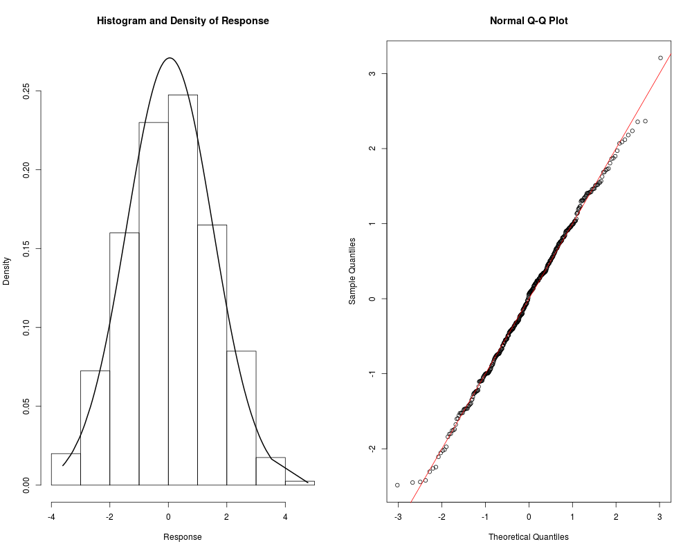
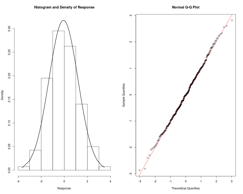
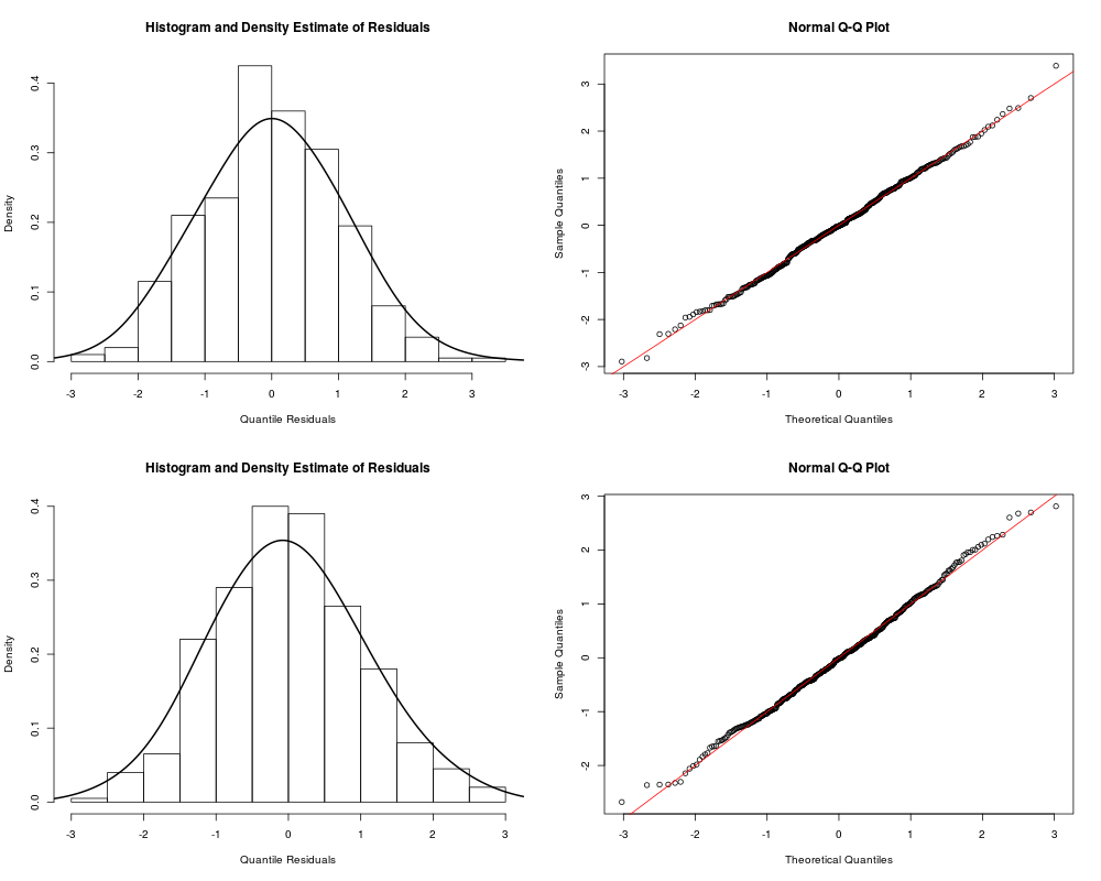
Examples

library(SemiParBIVProbit)

############
## Generate data
## Correlation between the two equations 0.5 - Sample size 400 

set.seed(0)

n <- 400

Sigma <- matrix(0.5, 2, 2); diag(Sigma) <- 1
u     <- rMVN(n, rep(0,2), Sigma)

x1 <- round(runif(n)); x2 <- runif(n); x3 <- runif(n)

f1   <- function(x) cos(pi*2*x) + sin(pi*x)
f2   <- function(x) x+exp(-30*(x-0.5)^2)   

y1 <- -1.55 + 2*x1    + f1(x2) + u[,1]
y2 <- -0.25 - 1.25*x1 + f2(x2) + u[,2]

dataSim <- data.frame(y1, y2, x1, x2, x3)

resp.check(y1, "N")
resp.check(y2, "N")

eq.mu.1     <- y1 ~ x1 + s(x2) + s(x3)
eq.mu.2     <- y2 ~ x1 + s(x2) + s(x3)
eq.sigma2.1 <-    ~ 1
eq.sigma2.2 <-    ~ 1
eq.theta    <-    ~ x1

fl <- list(eq.mu.1, eq.mu.2, eq.sigma2.1, eq.sigma2.2, eq.theta)

# the order above is the one to follow when
# using more than two equations

out  <- copulaReg(fl, data = dataSim)
conv.check(out)
post.check(out)
summary(out)
AIC(out)
BIC(out)
jc.probs(out, 1.4, 2.3, intervals = TRUE)[1:4,]

Results

R version 3.3.1 (2016-06-21) -- "Bug in Your Hair"
Copyright (C) 2016 The R Foundation for Statistical Computing
Platform: x86_64-pc-linux-gnu (64-bit)

R is free software and comes with ABSOLUTELY NO WARRANTY.
You are welcome to redistribute it under certain conditions.
Type 'license()' or 'licence()' for distribution details.

R is a collaborative project with many contributors.
Type 'contributors()' for more information and
'citation()' on how to cite R or R packages in publications.

Type 'demo()' for some demos, 'help()' for on-line help, or
'help.start()' for an HTML browser interface to help.
Type 'q()' to quit R.

> library(SemiParBIVProbit)
Loading required package: mgcv
Loading required package: nlme
This is mgcv 1.8-12. For overview type 'help("mgcv-package")'.

This is SemiParBIVProbit 3.7-1.
For overview type 'help("SemiParBIVProbit-package")'.

> png(filename="/home/ddbj/snapshot/RGM3/R_CC/result/SemiParBIVProbit/copulaReg.Rd_%03d_medium.png", width=480, height=480)
> ### Name: copulaReg
> ### Title: Semiparametric Copula Bivariate Models with Continuous Margins
> ### Aliases: copulaReg
> ### Keywords: semiparametric bivariate modelling smooth regression spline
> ###   shrinkage smoother variable selection copula
> 
> ### ** Examples
> 
> 
> library(SemiParBIVProbit)
> 
> ############
> ## Generate data
> ## Correlation between the two equations 0.5 - Sample size 400 
> 
> set.seed(0)
> 
> n <- 400
> 
> Sigma <- matrix(0.5, 2, 2); diag(Sigma) <- 1
> u     <- rMVN(n, rep(0,2), Sigma)
> 
> x1 <- round(runif(n)); x2 <- runif(n); x3 <- runif(n)
> 
> f1   <- function(x) cos(pi*2*x) + sin(pi*x)
> f2   <- function(x) x+exp(-30*(x-0.5)^2)   
> 
> y1 <- -1.55 + 2*x1    + f1(x2) + u[,1]
> y2 <- -0.25 - 1.25*x1 + f2(x2) + u[,2]
> 
> dataSim <- data.frame(y1, y2, x1, x2, x3)
> 
> resp.check(y1, "N")
> resp.check(y2, "N")
> 
> eq.mu.1     <- y1 ~ x1 + s(x2) + s(x3)
> eq.mu.2     <- y2 ~ x1 + s(x2) + s(x3)
> eq.sigma2.1 <-    ~ 1
> eq.sigma2.2 <-    ~ 1
> eq.theta    <-    ~ x1
> 
> fl <- list(eq.mu.1, eq.mu.2, eq.sigma2.1, eq.sigma2.2, eq.theta)
> 
> # the order above is the one to follow when
> # using more than two equations
> 
> out  <- copulaReg(fl, data = dataSim)
> conv.check(out)

Largest absolute gradient value: 2.567875e-10
Observed information matrix is positive definite
Eigenvalue range: [0.3597911,5.893766e+12]

Trust region iterations before smoothing parameter estimation: 7
Loops for smoothing parameter estimation: 4
Trust region iterations within smoothing loops: 8 

> post.check(out)
> summary(out)

COPULA:   Gaussian
MARGIN 1: Gaussian
MARGIN 2: Gaussian

EQUATION 1
Link function for mu.1: identity 
Formula: y1 ~ x1 + s(x2) + s(x3)

Parametric coefficients:
            Estimate Std. Error z value Pr(>|z|)    
(Intercept) -0.94817    0.06782  -13.98   <2e-16 ***
x1           2.04422    0.09726   21.02   <2e-16 ***
---
Signif. codes:  0 '***' 0.001 '**' 0.01 '*' 0.05 '.' 0.1 ' ' 1

Smooth components' approximate significance:
        edf Ref.df Chi.sq  p-value    
s(x2) 4.233  5.198 82.342 5.79e-16 ***
s(x3) 1.000  1.000  1.094    0.296    
---
Signif. codes:  0 '***' 0.001 '**' 0.01 '*' 0.05 '.' 0.1 ' ' 1


EQUATION 2
Link function for mu.2: identity 
Formula: y2 ~ x1 + s(x2) + s(x3)

Parametric coefficients:
            Estimate Std. Error z value Pr(>|z|)    
(Intercept)  0.51279    0.06948   7.381 1.58e-13 ***
x1          -1.18921    0.09967 -11.931  < 2e-16 ***
---
Signif. codes:  0 '***' 0.001 '**' 0.01 '*' 0.05 '.' 0.1 ' ' 1

Smooth components' approximate significance:
        edf Ref.df Chi.sq p-value    
s(x2) 5.354  6.465  94.24  <2e-16 ***
s(x3) 1.648  2.047   1.15   0.559    
---
Signif. codes:  0 '***' 0.001 '**' 0.01 '*' 0.05 '.' 0.1 ' ' 1


EQUATION 3
Link function for sigma2.1: log 
Formula: ~1

Parametric coefficients:
            Estimate Std. Error z value Pr(>|z|)
(Intercept) -0.06117    0.07055  -0.867    0.386


EQUATION 4
Link function for sigma2.2: log 
Formula: ~1

Parametric coefficients:
            Estimate Std. Error z value Pr(>|z|)
(Intercept) -0.01360    0.07093  -0.192    0.848


EQUATION 5
Link function for theta: atanh 
Formula: ~x1

Parametric coefficients:
            Estimate Std. Error z value Pr(>|z|)    
(Intercept)  0.52233    0.06691   7.806 5.89e-15 ***
x1           0.16435    0.08970   1.832   0.0669 .  
---
Signif. codes:  0 '***' 0.001 '**' 0.01 '*' 0.05 '.' 0.1 ' ' 1

sigma2.1 = 0.941(0.817,1.05)  sigma2.2 = 0.986(0.857,1.12)
theta = 0.536(0.441,0.613)  tau = 0.361(0.292,0.421)
n = 400  total edf = 20.2

> AIC(out)
[1] 2141.786
> BIC(out)
[1] 2222.554
> jc.probs(out, 1.4, 2.3, intervals = TRUE)[1:4,]
        p12      2.5%     97.5%        p1        p2
1 0.9335214 0.9015707 0.9603198 0.9979444 0.9345447
2 0.9411395 0.9074917 0.9732869 0.9693268 0.9655245
3 0.9084962 0.8476236 0.9587160 0.9579204 0.9388188
4 0.9477070 0.9070867 0.9723196 0.9797386 0.9631072
> 
> 
> 
> 
> 
> 
> 
> dev.off()
null device 
          1 
>