Semiparametric Sample Selection Modelling with Continuous or Discrete Response

Description

SemiParSampleSel can be used to fit continuous or discrete response sample selection models where the linear predictors are flexibly specified using parametric and regression spline components. The depedence between the selection and outcome equations is modelled through the use of copulas. Regression spline bases are extracted from the package mgcv. Multi-dimensional smooths are available via the use of penalized thin plate regression splines. If it makes sense, the dependence parameter of the chosen bivariate distribution as well as the shape and dispersion parameters of the outcome distribution can be specified as functions of semiparametric predictors.

Usage

SemiParSampleSel(formula, data = list(), weights = NULL, subset = NULL, 
                  start.v = NULL, start.theta = NULL,
                  BivD = "N", margins = c("probit","N"), fp = FALSE, infl.fac = 1,  
                  rinit = 1, rmax = 100, iterlimsp = 50, pr.tolsp = 1e-6, bd = NULL,
                  parscale)

Arguments

Details

The association between the responses is modelled by parameter ρ or θ. In a semiparametric bivariate sample selection model the linear predictors are flexibly specified using parametric components and smooth functions of covariates. Replacing the smooth components with their regression spline expressions yields a fully parametric bivariate sample selection model. In principle, classic maximum likelihood estimation can be employed. However, to avoid overfitting, penalized likelihood maximization is used instead. Here the use of penalty matrices allows for the suppression of that part of smooth term complexity which has no support from the data. The tradeoff between smoothness and fitness is controlled by smoothing parameters associated with the penalty matrices. Smoothing parameters are chosen to minimize the approximate Un-Biased Risk Estimator (UBRE) score, which can also be viewed as an approximate AIC.

The optimization problem is solved by a trust region algorithm. Automatic smoothing parameter selection is integrated using a performance-oriented iteration approach (Gu, 1992; Wood, 2004). Roughly speaking, at each iteration, (i) the penalized weighted least squares problem is solved, and (ii) the smoothing parameters of that problem estimated by approximate UBRE. Steps (i) and (ii) are iterated until convergence. Details of the underlying fitting methods are given in Marra and Radice (2013) and Wojtys et. al (in press).

Value

The function returns an object of class SemiParSampleSel as described in SemiParSampleSelObject.

WARNINGS

Convergence failure may occur when ρ or θ is very high, and/or the total number and selected number of observations are low, and/or there are important mistakes in the model specification (i.e., using C90 when the model equations are positively associated), and/or there are many smooth components in the model as compared to the number of observations. Convergence failure may also mean that an infinite cycling between steps (i) and (ii) occurs. In this case, the smoothing parameters are set to the values obtained from the non-converged algorithm (conv.check will give a warning). In such cases, we recommend re-specifying the model, and/or using some rescaling (see parscale).

In the context of non-random sample selection, it would not make much sense to specify the dependence parameter as function of covariates. This is because the assumption is that the dependence parameter models the association between the unobserved confounders in the two equations. However, this option does make sense when it is believed that the association coefficient varies across geographical areas, for instance.

Author(s)

Maintainer: Giampiero Marra giampiero.marra@ucl.ac.uk

References

Gu C. (1992), Cross validating non-Gaussian data. Journal of Computational and Graphical Statistics, 1(2), 169-179.

Marra G. and Radice R. (2013), Estimation of a Regression Spline Sample Selection Model. Computational Statistics and Data Analysis, 61, 158-173.

Wojtys M., Marra G. and Radice R. (in press), Copula Regression Spline Sample Selection Models: The R Package SemiParSampleSel. Journal of Statistical Software.

Wood S.N. (2004), Stable and efficient multiple smoothing parameter estimation for generalized additive models. Journal of the American Statistical Association, 99(467), 673-686.

See Also

aver, plot.SemiParSampleSel, SemiParSampleSel-package, SemiParSampleSelObject, conv.check, predict.SemiParSampleSel, summary.SemiParSampleSel

Examples

library(SemiParSampleSel)

######################################################################
## Generate data
## Correlation between the two equations and covariate correlation 0.5 
## Sample size 2000 
######################################################################

set.seed(0)

n <- 2000

rhC <- rhU <- 0.5      

SigmaU <- matrix(c(1, rhU, rhU, 1), 2, 2)
U      <- rmvnorm(n, rep(0,2), SigmaU)

SigmaC <- matrix(rhC, 3, 3); diag(SigmaC) <- 1

cov    <- rmvnorm(n, rep(0,3), SigmaC, method = "svd")
cov    <- pnorm(cov)

bi <- round(cov[,1]); x1 <- cov[,2]; x2 <- cov[,3]
  
f11 <- function(x) -0.7*(4*x + 2.5*x^2 + 0.7*sin(5*x) + cos(7.5*x))
f12 <- function(x) -0.4*( -0.3 - 1.6*x + sin(5*x))  
f21 <- function(x) 0.6*(exp(x) + sin(2.9*x)) 

ys <-  0.58 + 2.5*bi + f11(x1) + f12(x2) + U[, 1] > 0
y  <- -0.68 - 1.5*bi + f21(x1) +         + U[, 2]
yo <- y*(ys > 0)
  

dataSim <- data.frame(ys, yo, bi, x1, x2)

## CLASSIC SAMPLE SELECTION MODEL
## the first equation MUST be the selection equation

out <- SemiParSampleSel(list(ys ~ bi + x1 + x2, 
                             yo ~ bi + x1), 
                        data = dataSim)
conv.check(out)
summary(out)

AIC(out)
BIC(out)
aver(out)


## SEMIPARAMETRIC SAMPLE SELECTION MODEL

## "cr" cubic regression spline basis      - "cs" shrinkage version of "cr"
## "tp" thin plate regression spline basis - "ts" shrinkage version of "tp"
## for smooths of one variable, "cr/cs" and "tp/ts" achieve similar results 
## k is the basis dimension - default is 10
## m is the order of the penalty for the specific term - default is 2

out <- SemiParSampleSel(list(ys ~ bi + s(x1, bs = "tp", k = 10, m = 2) + s(x2), 
                             yo ~ bi + s(x1)), 
                        data = dataSim)
conv.check(out)                        
AIC(out)
aver(out)

## compare the two summary outputs
## the second output produces a summary of the results obtained when only 
## the outcome equation is fitted, i.e. selection bias is not accounted for

summary(out)
summary(out$gam2)

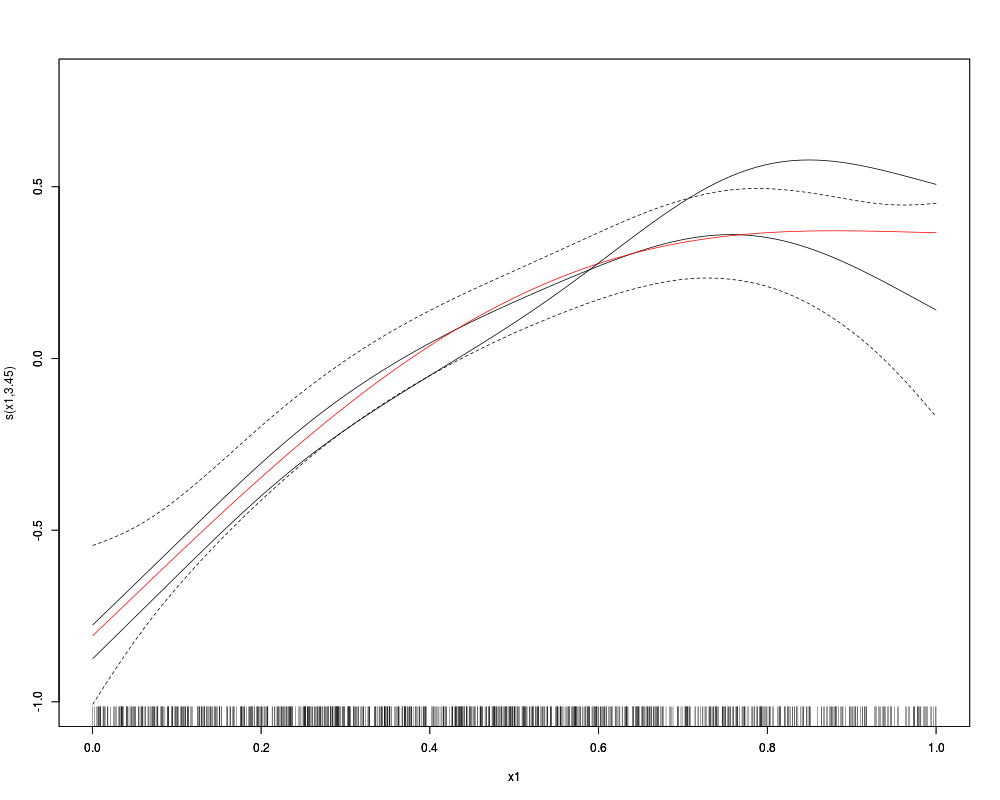
## estimated smooth function plots
## the red line is the true curve
## the blue line is the naive curve not accounting for selection bias

x1.s <- sort(x1[dataSim$ys>0])
f21.x1 <- f21(x1.s)[order(x1.s)] - mean(f21(x1.s))

plot(out, eq = 2, ylim = c(-1, 0.8)); lines(x1.s, f21.x1, col = "red")
par(new = TRUE)
plot(out$gam2, se = FALSE, col = "blue", ylim = c(-1, 0.8), ylab = "", rug = FALSE)




## Not run:  

## SEMIPARAMETRIC SAMPLE SELECTION MODEL with association and dispersion parameters 
## depending on covariates as well

out <- SemiParSampleSel(list(ys ~ bi + s(x1) + s(x2), 
                             yo ~ bi + s(x1),
                                ~ bi, 
                                ~ bi + x1), 
                        data = dataSim)
conv.check(out)                        
summary(out)
out$sigma
out$theta

#
#

###################################################
## example using Clayton copula with normal margins
###################################################

set.seed(0)

theta <- 5
sig  <- 1.5

myCop <- archmCopula(family = "clayton", dim = 2, param = theta)

# other copula options are for instance: "amh", "frank", "gumbel", "joe"
# for FGM use the following code:
# myCop <- fgmCopula(theta, dim=2)

bivg  <- mvdc(copula = myCop, c("norm", "norm"), 
              list(list(mean = 0, sd = 1), 
              list(mean = 0, sd = sig)))
er    <- rMvdc(n, bivg)

ys <-  0.58 + 2.5*bi + f11(x1) + f12(x2) + er[, 1] > 0
y  <- -0.68 - 1.5*bi + f21(x1) +         + er[, 2]
yo <- y*(ys > 0)
  
dataSim <- data.frame(ys, yo, bi, x1, x2)

out <- SemiParSampleSel(list(ys ~ bi + s(x1) + s(x2), 
                             yo ~ bi + s(x1)), 
                        data = dataSim, BivD = "C0")
conv.check(out)
summary(out)
aver(out)

x1.s <- sort(x1[dataSim$ys>0])
f21.x1 <- f21(x1.s)[order(x1.s)] - mean(f21(x1.s))

plot(out, eq = 2, ylim = c(-1.1, 1.6)); lines(x1.s, f21.x1, col = "red")
par(new = TRUE)
plot(out$gam2, se = FALSE, col = "blue", ylim = c(-1.1, 1.6), ylab = "", rug = FALSE)

#
#

########################################################
## example using Gumbel copula with normal-gamma margins
########################################################

set.seed(0)

k <- 2                                # shape of gamma distribution
miu  <- exp(-0.68 - 1.5*bi + f21(x1)) # mean values of y's (log m = Xb)
lambda <- k/miu	                      # rate of gamma distribution

theta <- 6

# Two-dimensional Gumbel copula with unif margins
gumbel.cop <- onacopula("Gumbel", C(theta, 1:2))

# Random sample from two-dimensional Gumbel copula with uniform margins
U <- rnacopula(n = n, gumbel.cop)		  

# Margins: normal and gamma
er <- cbind(qnorm(U[,1], 0, 1), qgamma(U[, 2], shape = k, rate = lambda))

ys <- 0.58 + 2.5*bi + f11(x1) + f12(x2) + er[, 1] > 0
y  <- er[, 2]
yo <- y*(ys > 0)

dataSim <- data.frame(ys, yo, bi, x1, x2)

out <- SemiParSampleSel(list(ys ~ bi + s(x1) + s(x2), 
                             yo ~ bi + s(x1)), 
                        data = dataSim, BivD = "G0", margins = c("N", "G"))
conv.check(out)
summary(out)
aver(out)

x1.s <- sort(x1[dataSim$ys>0])
f21.x1 <- f21(x1.s)[order(x1.s)] - mean(f21(x1.s))

plot(out, eq = 2, ylim = c(-1.1, 1)); lines(x1.s, f21.x1, col = "red")
par(new = TRUE)
plot(out$gam2, se = FALSE, col = "blue", ylim = c(-1.1, 1), ylab = "", rug = FALSE)

#
#


########################################################
## Example for discrete margins and normal copula
########################################################


# Creating simulation function
bcds <- function(n, s.tau = 0.2, s.sigma = 1, s.nu = 0.5, 
                rhC = 0.2, outcome.margin = "PO", copula = "FGM")  {
  
# Generating covariates     
  SigmaC <- matrix( c(1,rhC,rhC,rhC,rhC,1,rhC,rhC,rhC,rhC,1,rhC,rhC,rhC,rhC,1), 4 , 4)
  covariates    <- rmvnorm(n,rep(0,4),SigmaC, method="svd")
  covariates    <- pnorm(covariates)
  x1 <- covariates[,1]
  x2 <- covariates[,2]
  x3 <- round(covariates[,3])
  x4 <- round(covariates[,4])
  
  # Establishing copula object
  if (copula == "FGM") {
      Cop <- fgmCopula(dim = 2, param = iTau(fgmCopula(), s.tau))
    } else if (copula == "N") {
      Cop <- ellipCopula(family = "normal", dim = 2, param = iTau(normalCopula(), s.tau))
    } else if (copula == "AMH") {
      Cop <- archmCopula(family = "amh", dim = 2, param = iTau(amhCopula(), s.tau))
    } else if (copula == "C0") {
      Cop <- archmCopula(family = "clayton", dim = 2, param = iTau(claytonCopula(), s.tau))
    } else if (copula == "F") {
      Cop <- archmCopula(family = "frank", dim = 2, param = iTau(frankCopula(), s.tau))
    } else if (copula == "G0") {
      Cop <- archmCopula(family = "gumbel", dim = 2, param = iTau(gumbelCopula(), s.tau))
    } else if (copula == "J0") {
      Cop <- archmCopula(family = "joe", dim = 2, param = iTau(joeCopula(), s.tau))
    }  
  
  # Setting up equations
  f1 <- function(x) 0.4*(-4 - (5.5*x-2.9) + 3*(4.5*x-2.3)^2 - (4.5*x-2.3)^3)
  f2 <- function(x) x*sin(8*x)
  mu_s  <- 1.0 + f1(x1) - 2.0*x2 + 3.1*x3 - 2.2*x4
  mu_o  <-  exp(1.3 + f2(x1) - 1.9*x2 + 2.4*x3 - 0.1*x4)
  
  # Creating margin dependent object
  if (outcome.margin == "P") {
        speclist <- list(mu = mu_o)
        outcome.margin2 <- "PO"
     } else if (outcome.margin == "NB") {
        speclist  <- list(mu = mu_o, sigma = s.sigma)
        outcome.margin2 <- "NBI"
     } else if (outcome.margin == "D") {
        speclist  <- list(mu = mu_o, sigma = s.sigma, nu = s.nu)
        outcome.margin2 <- "DEL"
     } else if (outcome.margin == "PIG") {
        speclist  <- list(mu = mu_o, sigma = s.sigma)
        outcome.margin2 <- "PIG"
     } else if (outcome.margin == "S") {
        speclist  <- list(mu = mu_o, sigma = s.sigma, nu = s.nu)
        outcome.margin2 <- "SICHEL"
   }
  spec  <- mvdc(copula = Cop, c("norm", outcome.margin2), 
                list(list(mean = mu_s, sd = 1), speclist))  
  
  # Simulating data
  simGen <- rMvdc(n, spec)
  y <- ifelse(simGen[,1]>0, simGen[,2], -99)
  
  dataSim <- data.frame(y, x1, x2, x3, x4)  
  dataSim  
}



# Creating plots of the true functional form of x1 in both equations
xt1  <- seq(0, 1, length.out=200)
xt2  <- seq(0,1, length.out=200)
f1t <- function(x) 0.4*(-4 - (5.5*x-2.9) + 3*(4.5*x-2.3)^2 - (4.5*x-2.3)^3)
f2t <- function(x) x*sin(8*x)
plot(xt1, f1t(xt1))
plot(xt2, f2t(xt2))




# Simulating 1000 deviates

set.seed(0)

dataSim<- bcds(1000, s.tau = 0.6, s.sigma = 0.1, s.nu = 0.5, 
                rhC = 0.5, outcome.margin = "NB", copula = "N")
dataSim$y.probit<-ifelse(dataSim$y >= 0, 1, 0)


# Estimating SemiParSampleSel

out1 <- SemiParSampleSel(list(y.probit ~ s(x1) + x2 + x3 + x4, y ~ s(x1) + x2 + x3 + x4), 
                          data = dataSim, BivD = "N", margins = c("N", "P")) 
conv.check(out1)

out2 <- SemiParSampleSel(list(y.probit ~ s(x1) + x2 + x3 + x4, y ~ s(x1) + x2 + x3 + x4), 
                         data = dataSim, BivD = "N", margins = c("N", "NB")) 
conv.check(out2)


# Model comparison

AIC(out1)
AIC(out2)
VuongClarke(out1, out2)


# Model diagnostics

summary(out2, cm.plot = TRUE)
plot(out2, eq = 1)
plot(out2, eq = 2)
aver(out2, univariate = TRUE)
aver(out2, univariate = FALSE)

#
#



## End(Not run)

Results

R version 3.3.1 (2016-06-21) -- "Bug in Your Hair"
Copyright (C) 2016 The R Foundation for Statistical Computing
Platform: x86_64-pc-linux-gnu (64-bit)

R is free software and comes with ABSOLUTELY NO WARRANTY.
You are welcome to redistribute it under certain conditions.
Type 'license()' or 'licence()' for distribution details.

R is a collaborative project with many contributors.
Type 'contributors()' for more information and
'citation()' on how to cite R or R packages in publications.

Type 'demo()' for some demos, 'help()' for on-line help, or
'help.start()' for an HTML browser interface to help.
Type 'q()' to quit R.

> library(SemiParSampleSel)
Loading required package: copula
Loading required package: mgcv
Loading required package: nlme
This is mgcv 1.8-12. For overview type 'help("mgcv-package")'.
Loading required package: mvtnorm
Loading required package: gamlss.dist
Loading required package: MASS

This is SemiParSampleSel 1.3.
For overview type 'help("SemiParSampleSel-package")'.

> png(filename="/home/ddbj/snapshot/RGM3/R_CC/result/SemiParSampleSel/SemiParSampleSel.Rd_%03d_medium.png", width=480, height=480)
> ### Name: SemiParSampleSel
> ### Title: Semiparametric Sample Selection Modelling with Continuous or
> ###   Discrete Response
> ### Aliases: SemiParSampleSel
> ### Keywords: copula sample selection semiparametric sample selection
> ###   modelling sample selection model smooth regression spline shrinkage
> ###   smoother variable selection
> 
> ### ** Examples
> 
> 
> library(SemiParSampleSel)
> 
> ######################################################################
> ## Generate data
> ## Correlation between the two equations and covariate correlation 0.5 
> ## Sample size 2000 
> ######################################################################
> 
> set.seed(0)
> 
> n <- 2000
> 
> rhC <- rhU <- 0.5      
> 
> SigmaU <- matrix(c(1, rhU, rhU, 1), 2, 2)
> U      <- rmvnorm(n, rep(0,2), SigmaU)
> 
> SigmaC <- matrix(rhC, 3, 3); diag(SigmaC) <- 1
> 
> cov    <- rmvnorm(n, rep(0,3), SigmaC, method = "svd")
> cov    <- pnorm(cov)
> 
> bi <- round(cov[,1]); x1 <- cov[,2]; x2 <- cov[,3]
>   
> f11 <- function(x) -0.7*(4*x + 2.5*x^2 + 0.7*sin(5*x) + cos(7.5*x))
> f12 <- function(x) -0.4*( -0.3 - 1.6*x + sin(5*x))  
> f21 <- function(x) 0.6*(exp(x) + sin(2.9*x)) 
> 
> ys <-  0.58 + 2.5*bi + f11(x1) + f12(x2) + U[, 1] > 0
> y  <- -0.68 - 1.5*bi + f21(x1) +         + U[, 2]
> yo <- y*(ys > 0)
>   
> 
> dataSim <- data.frame(ys, yo, bi, x1, x2)
> 
> ## CLASSIC SAMPLE SELECTION MODEL
> ## the first equation MUST be the selection equation
> 
> out <- SemiParSampleSel(list(ys ~ bi + x1 + x2, 
+                              yo ~ bi + x1), 
+                         data = dataSim)
> conv.check(out)

Largest absolute gradient value: 2.505222e-09
Observed information matrix is positive definite
Eigenvalue range: [17.62329,2509.637]

Trust region iterations: 4 

> summary(out)

ERRORS' DISTRIBUTION: Bivariate Normal

SELECTION EQ.
Family: Bernoulli
Link function: probit
Formula: ys ~ bi + x1 + x2

            Estimate Std. Error z value Pr(>|z|)    
(Intercept)  0.01756    0.07206   0.244    0.807    
bi           2.30297    0.10621  21.683   <2e-16 ***
x1          -3.99821    0.20360 -19.638   <2e-16 ***
x2           1.69695    0.14950  11.351   <2e-16 ***
---
Signif. codes:  0 '***' 0.001 '**' 0.01 '*' 0.05 '.' 0.1 ' ' 1

OUTCOME EQ.
Family: Gaussian
Link function: identity
Formula: yo ~ bi + x1

            Estimate Std. Error z value Pr(>|z|)    
(Intercept)   0.3753     0.1011   3.712 0.000206 ***
bi           -1.6488     0.1279 -12.890  < 2e-16 ***
x1            1.1208     0.1687   6.645 3.03e-11 ***
---
Signif. codes:  0 '***' 0.001 '**' 0.01 '*' 0.05 '.' 0.1 ' ' 1

n = 2000  n.sel = 1022  sigma = 0.997(0.943,1.057)
theta = 0.418(0.221,0.586)  total edf = 9

> 
> AIC(out)
[1] 4589.734
> BIC(out)
[1] 4640.142
> aver(out)

Estimated average with 95% confidence interval:

0.0828 (-0.0164,0.1819)

> 
> 
> ## SEMIPARAMETRIC SAMPLE SELECTION MODEL
> 
> ## "cr" cubic regression spline basis      - "cs" shrinkage version of "cr"
> ## "tp" thin plate regression spline basis - "ts" shrinkage version of "tp"
> ## for smooths of one variable, "cr/cs" and "tp/ts" achieve similar results 
> ## k is the basis dimension - default is 10
> ## m is the order of the penalty for the specific term - default is 2
> 
> out <- SemiParSampleSel(list(ys ~ bi + s(x1, bs = "tp", k = 10, m = 2) + s(x2), 
+                              yo ~ bi + s(x1)), 
+                         data = dataSim)
> conv.check(out)                        

Largest absolute gradient value: 5.166329e-06
Observed information matrix is positive definite
Eigenvalue range: [0.7221395,7718.65]

Trust region iterations before smoothing parameter estimation: 4
Loops for smoothing parameter estimation: 4
Trust region iterations within smoothing loops: 7 

> AIC(out)
[1] 4453.923
> aver(out)

Estimated average with 95% confidence interval:

0.0451 (-0.0386,0.1287)

> 
> ## compare the two summary outputs
> ## the second output produces a summary of the results obtained when only 
> ## the outcome equation is fitted, i.e. selection bias is not accounted for
> 
> summary(out)

ERRORS' DISTRIBUTION: Bivariate Normal

SELECTION EQ.
Family: Bernoulli
Link function: probit
Formula: ys ~ bi + s(x1, bs = "tp", k = 10, m = 2) + s(x2)

            Estimate Std. Error z value Pr(>|z|)    
(Intercept) -1.26575    0.07143  -17.72   <2e-16 ***
bi           2.63268    0.13290   19.81   <2e-16 ***
---
Signif. codes:  0 '***' 0.001 '**' 0.01 '*' 0.05 '.' 0.1 ' ' 1

Smooth components' approximate significance:
        edf Ref.df Chi.sq p-value    
s(x1) 5.299  6.427  383.3  <2e-16 ***
s(x2) 3.630  4.501  156.5  <2e-16 ***
---
Signif. codes:  0 '***' 0.001 '**' 0.01 '*' 0.05 '.' 0.1 ' ' 1

OUTCOME EQ.
Family: Gaussian
Link function: identity
Formula: yo ~ bi + s(x1)

            Estimate Std. Error z value Pr(>|z|)    
(Intercept)   0.8695     0.1243   6.993 2.69e-12 ***
bi           -1.6369     0.1178 -13.896  < 2e-16 ***
---
Signif. codes:  0 '***' 0.001 '**' 0.01 '*' 0.05 '.' 0.1 ' ' 1

Smooth components' approximate significance:
        edf Ref.df Chi.sq  p-value    
s(x1) 3.452  4.297  79.44 6.95e-16 ***
---
Signif. codes:  0 '***' 0.001 '**' 0.01 '*' 0.05 '.' 0.1 ' ' 1

n = 2000  n.sel = 1022  sigma = 0.996(0.944,1.051)
theta = 0.476(0.308,0.62)  total edf = 18.381

> summary(out$gam2)

Family: gaussian 
Link function: identity 

Formula:
yo ~ bi + s(x1)

Parametric coefficients:
            Estimate Std. Error t value Pr(>|t|)    
(Intercept)  1.41565    0.06659   21.26   <2e-16 ***
bi          -2.08466    0.07957  -26.20   <2e-16 ***
---
Signif. codes:  0 '***' 0.001 '**' 0.01 '*' 0.05 '.' 0.1 ' ' 1

Approximate significance of smooth terms:
       edf Ref.df     F p-value    
s(x1) 3.83  4.743 32.31  <2e-16 ***
---
Signif. codes:  0 '***' 0.001 '**' 0.01 '*' 0.05 '.' 0.1 ' ' 1

R-sq.(adj) =  0.404   Deviance explained = 40.7%
GCV = 0.93013  Scale est. = 0.92483   n = 1022
> 
> ## estimated smooth function plots
> ## the red line is the true curve
> ## the blue line is the naive curve not accounting for selection bias
> 
> x1.s <- sort(x1[dataSim$ys>0])
> f21.x1 <- f21(x1.s)[order(x1.s)] - mean(f21(x1.s))
> 
> plot(out, eq = 2, ylim = c(-1, 0.8)); lines(x1.s, f21.x1, col = "red")
> par(new = TRUE)
> plot(out$gam2, se = FALSE, col = "blue", ylim = c(-1, 0.8), ylab = "", rug = FALSE)
> 
> 
> 
> 
> ## Not run: 
> ##D  
> ##D 
> ##D ## SEMIPARAMETRIC SAMPLE SELECTION MODEL with association and dispersion parameters 
> ##D ## depending on covariates as well
> ##D 
> ##D out <- SemiParSampleSel(list(ys ~ bi + s(x1) + s(x2), 
> ##D                              yo ~ bi + s(x1),
> ##D                                 ~ bi, 
> ##D                                 ~ bi + x1), 
> ##D                         data = dataSim)
> ##D conv.check(out)                        
> ##D summary(out)
> ##D out$sigma
> ##D out$theta
> ##D 
> ##D #
> ##D #
> ##D 
> ##D ###################################################
> ##D ## example using Clayton copula with normal margins
> ##D ###################################################
> ##D 
> ##D set.seed(0)
> ##D 
> ##D theta <- 5
> ##D sig  <- 1.5
> ##D 
> ##D myCop <- archmCopula(family = "clayton", dim = 2, param = theta)
> ##D 
> ##D # other copula options are for instance: "amh", "frank", "gumbel", "joe"
> ##D # for FGM use the following code:
> ##D # myCop <- fgmCopula(theta, dim=2)
> ##D 
> ##D bivg  <- mvdc(copula = myCop, c("norm", "norm"), 
> ##D               list(list(mean = 0, sd = 1), 
> ##D               list(mean = 0, sd = sig)))
> ##D er    <- rMvdc(n, bivg)
> ##D 
> ##D ys <-  0.58 + 2.5*bi + f11(x1) + f12(x2) + er[, 1] > 0
> ##D y  <- -0.68 - 1.5*bi + f21(x1) +         + er[, 2]
> ##D yo <- y*(ys > 0)
> ##D   
> ##D dataSim <- data.frame(ys, yo, bi, x1, x2)
> ##D 
> ##D out <- SemiParSampleSel(list(ys ~ bi + s(x1) + s(x2), 
> ##D                              yo ~ bi + s(x1)), 
> ##D                         data = dataSim, BivD = "C0")
> ##D conv.check(out)
> ##D summary(out)
> ##D aver(out)
> ##D 
> ##D x1.s <- sort(x1[dataSim$ys>0])
> ##D f21.x1 <- f21(x1.s)[order(x1.s)] - mean(f21(x1.s))
> ##D 
> ##D plot(out, eq = 2, ylim = c(-1.1, 1.6)); lines(x1.s, f21.x1, col = "red")
> ##D par(new = TRUE)
> ##D plot(out$gam2, se = FALSE, col = "blue", ylim = c(-1.1, 1.6), ylab = "", rug = FALSE)
> ##D 
> ##D #
> ##D #
> ##D 
> ##D ########################################################
> ##D ## example using Gumbel copula with normal-gamma margins
> ##D ########################################################
> ##D 
> ##D set.seed(0)
> ##D 
> ##D k <- 2                                # shape of gamma distribution
> ##D miu  <- exp(-0.68 - 1.5*bi + f21(x1)) # mean values of y's (log m = Xb)
> ##D lambda <- k/miu	                      # rate of gamma distribution
> ##D 
> ##D theta <- 6
> ##D 
> ##D # Two-dimensional Gumbel copula with unif margins
> ##D gumbel.cop <- onacopula("Gumbel", C(theta, 1:2))
> ##D 
> ##D # Random sample from two-dimensional Gumbel copula with uniform margins
> ##D U <- rnacopula(n = n, gumbel.cop)		  
> ##D 
> ##D # Margins: normal and gamma
> ##D er <- cbind(qnorm(U[,1], 0, 1), qgamma(U[, 2], shape = k, rate = lambda))
> ##D 
> ##D ys <- 0.58 + 2.5*bi + f11(x1) + f12(x2) + er[, 1] > 0
> ##D y  <- er[, 2]
> ##D yo <- y*(ys > 0)
> ##D 
> ##D dataSim <- data.frame(ys, yo, bi, x1, x2)
> ##D 
> ##D out <- SemiParSampleSel(list(ys ~ bi + s(x1) + s(x2), 
> ##D                              yo ~ bi + s(x1)), 
> ##D                         data = dataSim, BivD = "G0", margins = c("N", "G"))
> ##D conv.check(out)
> ##D summary(out)
> ##D aver(out)
> ##D 
> ##D x1.s <- sort(x1[dataSim$ys>0])
> ##D f21.x1 <- f21(x1.s)[order(x1.s)] - mean(f21(x1.s))
> ##D 
> ##D plot(out, eq = 2, ylim = c(-1.1, 1)); lines(x1.s, f21.x1, col = "red")
> ##D par(new = TRUE)
> ##D plot(out$gam2, se = FALSE, col = "blue", ylim = c(-1.1, 1), ylab = "", rug = FALSE)
> ##D 
> ##D #
> ##D #
> ##D 
> ##D 
> ##D ########################################################
> ##D ## Example for discrete margins and normal copula
> ##D ########################################################
> ##D 
> ##D 
> ##D # Creating simulation function
> ##D bcds <- function(n, s.tau = 0.2, s.sigma = 1, s.nu = 0.5, 
> ##D                 rhC = 0.2, outcome.margin = "PO", copula = "FGM")  {
> ##D   
> ##D # Generating covariates     
> ##D   SigmaC <- matrix( c(1,rhC,rhC,rhC,rhC,1,rhC,rhC,rhC,rhC,1,rhC,rhC,rhC,rhC,1), 4 , 4)
> ##D   covariates    <- rmvnorm(n,rep(0,4),SigmaC, method="svd")
> ##D   covariates    <- pnorm(covariates)
> ##D   x1 <- covariates[,1]
> ##D   x2 <- covariates[,2]
> ##D   x3 <- round(covariates[,3])
> ##D   x4 <- round(covariates[,4])
> ##D   
> ##D   # Establishing copula object
> ##D   if (copula == "FGM") {
> ##D       Cop <- fgmCopula(dim = 2, param = iTau(fgmCopula(), s.tau))
> ##D     } else if (copula == "N") {
> ##D       Cop <- ellipCopula(family = "normal", dim = 2, param = iTau(normalCopula(), s.tau))
> ##D     } else if (copula == "AMH") {
> ##D       Cop <- archmCopula(family = "amh", dim = 2, param = iTau(amhCopula(), s.tau))
> ##D     } else if (copula == "C0") {
> ##D       Cop <- archmCopula(family = "clayton", dim = 2, param = iTau(claytonCopula(), s.tau))
> ##D     } else if (copula == "F") {
> ##D       Cop <- archmCopula(family = "frank", dim = 2, param = iTau(frankCopula(), s.tau))
> ##D     } else if (copula == "G0") {
> ##D       Cop <- archmCopula(family = "gumbel", dim = 2, param = iTau(gumbelCopula(), s.tau))
> ##D     } else if (copula == "J0") {
> ##D       Cop <- archmCopula(family = "joe", dim = 2, param = iTau(joeCopula(), s.tau))
> ##D     }  
> ##D   
> ##D   # Setting up equations
> ##D   f1 <- function(x) 0.4*(-4 - (5.5*x-2.9) + 3*(4.5*x-2.3)^2 - (4.5*x-2.3)^3)
> ##D   f2 <- function(x) x*sin(8*x)
> ##D   mu_s  <- 1.0 + f1(x1) - 2.0*x2 + 3.1*x3 - 2.2*x4
> ##D   mu_o  <-  exp(1.3 + f2(x1) - 1.9*x2 + 2.4*x3 - 0.1*x4)
> ##D   
> ##D   # Creating margin dependent object
> ##D   if (outcome.margin == "P") {
> ##D         speclist <- list(mu = mu_o)
> ##D         outcome.margin2 <- "PO"
> ##D      } else if (outcome.margin == "NB") {
> ##D         speclist  <- list(mu = mu_o, sigma = s.sigma)
> ##D         outcome.margin2 <- "NBI"
> ##D      } else if (outcome.margin == "D") {
> ##D         speclist  <- list(mu = mu_o, sigma = s.sigma, nu = s.nu)
> ##D         outcome.margin2 <- "DEL"
> ##D      } else if (outcome.margin == "PIG") {
> ##D         speclist  <- list(mu = mu_o, sigma = s.sigma)
> ##D         outcome.margin2 <- "PIG"
> ##D      } else if (outcome.margin == "S") {
> ##D         speclist  <- list(mu = mu_o, sigma = s.sigma, nu = s.nu)
> ##D         outcome.margin2 <- "SICHEL"
> ##D    }
> ##D   spec  <- mvdc(copula = Cop, c("norm", outcome.margin2), 
> ##D                 list(list(mean = mu_s, sd = 1), speclist))  
> ##D   
> ##D   # Simulating data
> ##D   simGen <- rMvdc(n, spec)
> ##D   y <- ifelse(simGen[,1]>0, simGen[,2], -99)
> ##D   
> ##D   dataSim <- data.frame(y, x1, x2, x3, x4)  
> ##D   dataSim  
> ##D }
> ##D 
> ##D 
> ##D 
> ##D # Creating plots of the true functional form of x1 in both equations
> ##D xt1  <- seq(0, 1, length.out=200)
> ##D xt2  <- seq(0,1, length.out=200)
> ##D f1t <- function(x) 0.4*(-4 - (5.5*x-2.9) + 3*(4.5*x-2.3)^2 - (4.5*x-2.3)^3)
> ##D f2t <- function(x) x*sin(8*x)
> ##D plot(xt1, f1t(xt1))
> ##D plot(xt2, f2t(xt2))
> ##D 
> ##D 
> ##D 
> ##D 
> ##D # Simulating 1000 deviates
> ##D 
> ##D set.seed(0)
> ##D 
> ##D dataSim<- bcds(1000, s.tau = 0.6, s.sigma = 0.1, s.nu = 0.5, 
> ##D                 rhC = 0.5, outcome.margin = "NB", copula = "N")
> ##D dataSim$y.probit<-ifelse(dataSim$y >= 0, 1, 0)
> ##D 
> ##D 
> ##D # Estimating SemiParSampleSel
> ##D 
> ##D out1 <- SemiParSampleSel(list(y.probit ~ s(x1) + x2 + x3 + x4, y ~ s(x1) + x2 + x3 + x4), 
> ##D                           data = dataSim, BivD = "N", margins = c("N", "P")) 
> ##D conv.check(out1)
> ##D 
> ##D out2 <- SemiParSampleSel(list(y.probit ~ s(x1) + x2 + x3 + x4, y ~ s(x1) + x2 + x3 + x4), 
> ##D                          data = dataSim, BivD = "N", margins = c("N", "NB")) 
> ##D conv.check(out2)
> ##D 
> ##D 
> ##D # Model comparison
> ##D 
> ##D AIC(out1)
> ##D AIC(out2)
> ##D VuongClarke(out1, out2)
> ##D 
> ##D 
> ##D # Model diagnostics
> ##D 
> ##D summary(out2, cm.plot = TRUE)
> ##D plot(out2, eq = 1)
> ##D plot(out2, eq = 2)
> ##D aver(out2, univariate = TRUE)
> ##D aver(out2, univariate = FALSE)
> ##D 
> ##D #
> ##D #
> ##D 
> ##D 
> ## End(Not run)
> 
> 
> 
> 
> 
> 
> dev.off()
null device 
          1 
>