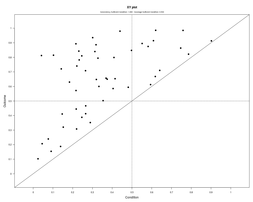
Function producing enhanced XY plots

Description

xy.plot produces xyplots and provides coverage and consistency values. The advantage over fsplot() (in the QCA3 package) is its larger flexibility and that it does not need a dataset to work, it just need two vectors. Several graphic parameters can be decided by the user.

Usage

xy.plot(x, y, 
        ylim = c(-0.05, 1.05), xlim = c(-0.05, 1.05), 
        pch = 19, col = "black", main = "XY plot", 
        ylab = "Outcome", xlab = "Condition", 
        mar = c(4, 4, 4, 1), mgp = c(2.2, 0.8, 0), 
        cex.fit = 0.6, cex.axis = 0.7, cex.main = 1, 
        necessity = FALSE, show.hv = TRUE, show.fit = TRUE, 
        pos.fit = "top", case.lab = TRUE, labs = NULL, 
        cex.lab = 0.8, offset.x = 0, offset.y = 0, 
        pos = 4, srt = 0, 
        ident = FALSE)

Arguments

Value

It returns an enhanced XY plot.

Author(s)

Mario Quaranta.

References

Ragin, C. C. (2008) Redesigning Social Inquiry: Fuzzy Sets and Beyond. The Chicago University Press: Chicago and London.

Schneider, C. Q., Wagemann, C. (2012) Set-Theoretic Methods for the Social Sciences, Cambridge Univeristy Press: Cambridge.

Schneider, C. Q., Wagemann, C., Quaranta, M. (2012) How To... Use Software for Set-Theoretic Analysis. Online Appendix to "Set-Theoretic Methods for the Social Sciences". Available at www.cambridge.org/schneider-wagemann

Examples

# Generate fake data
set.seed(123)
x <- runif(40, 0, 1)
y <- runif(40, 0, 1)

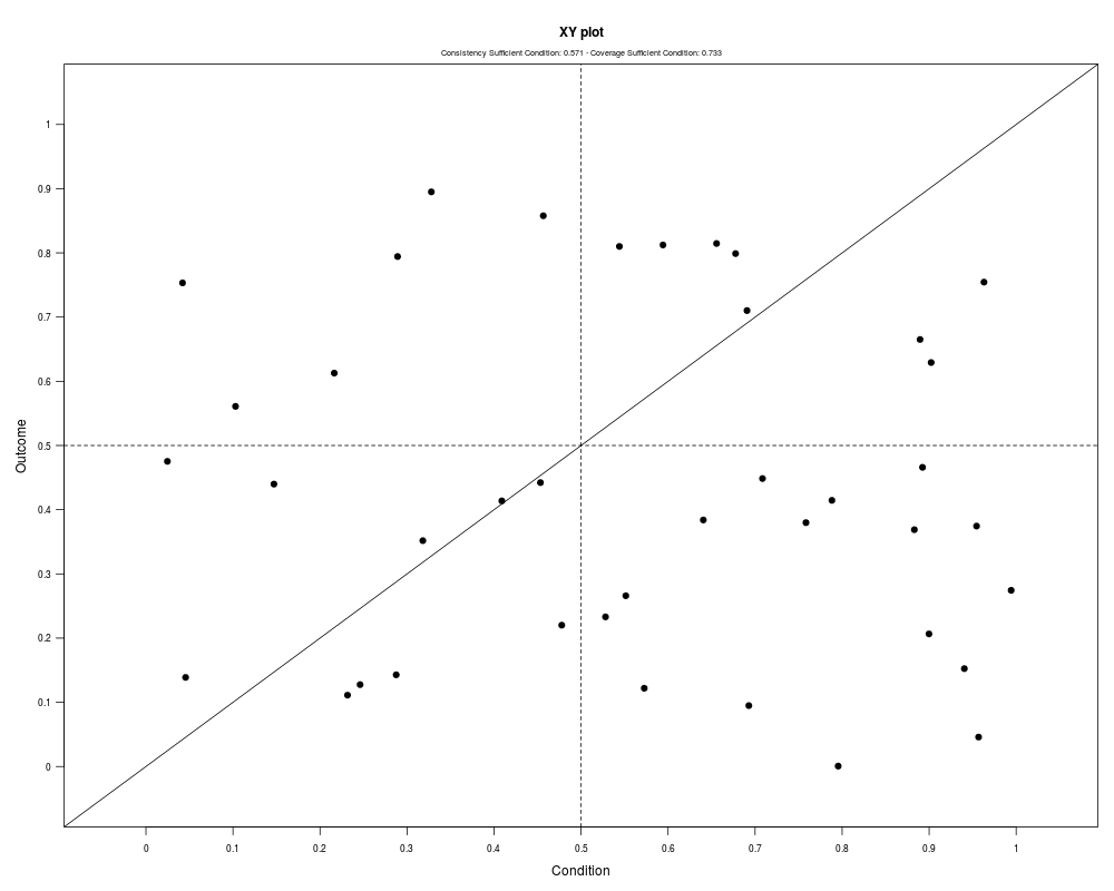
# Default
xy.plot(x, y)

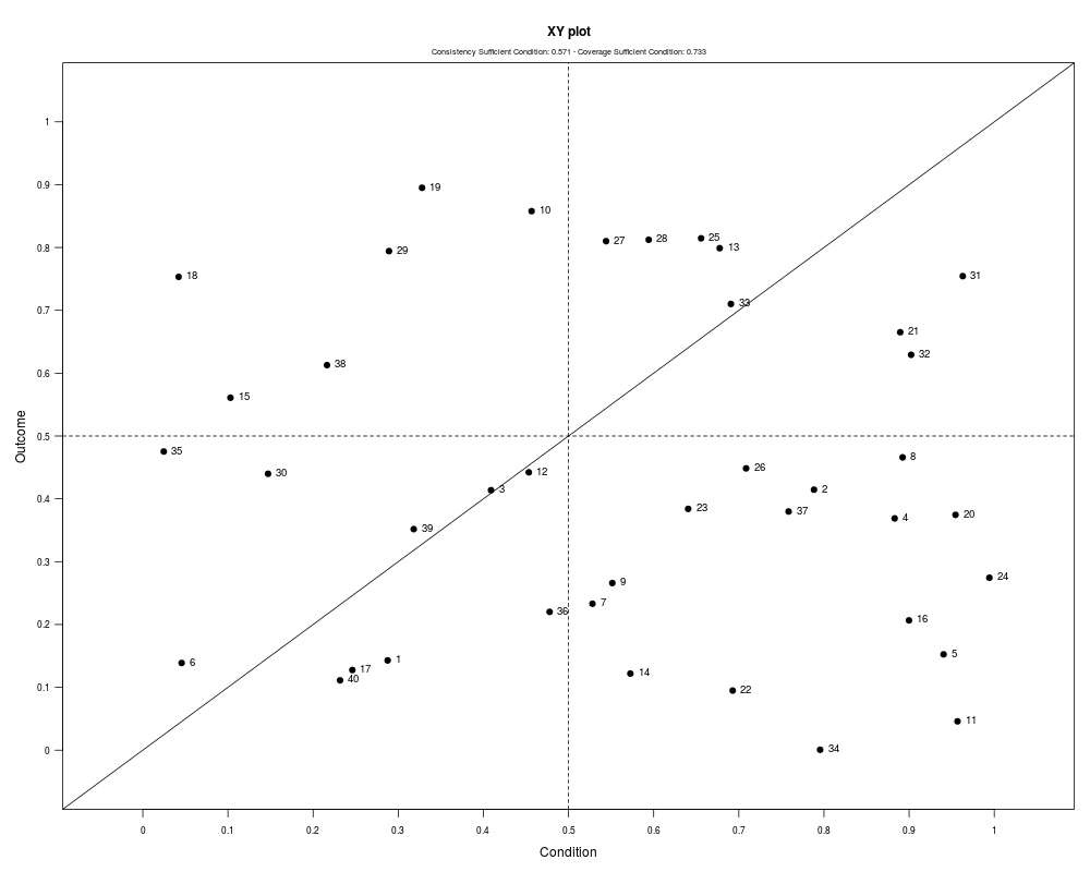
# With labels
xy.plot(x, y, case.lab = TRUE, labs = 1:40)

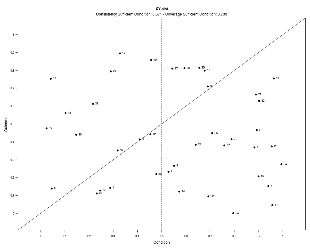
# With labels and bigger measures of fit
xy.plot(x, y, case.lab = TRUE, labs = 1:40, cex.fit = 1)

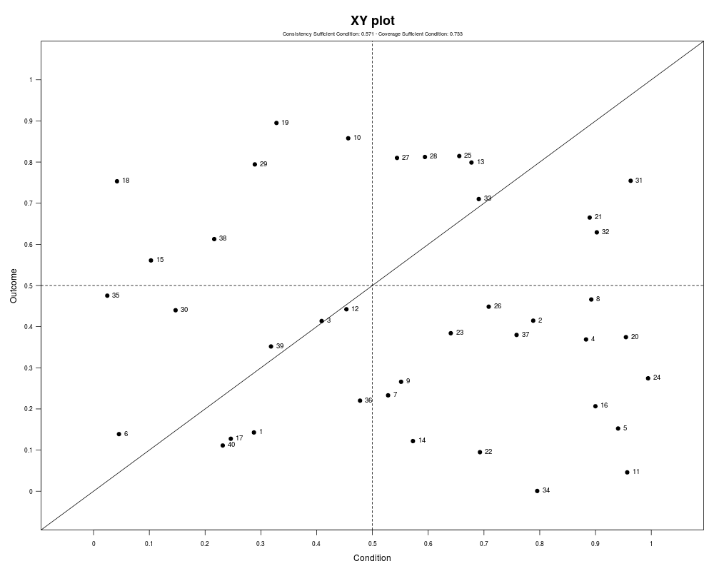
# With labels and bigger title
xy.plot(x, y, case.lab = TRUE, labs = 1:40, cex.main = 1.5)

# Generate fake data the have perfect sufficiency
set.seed(123)
x <- runif(50, 0, 1)
y <- runif(50, 0, 1)

for(i in 1:length(y)) {
    while(x[i] > y[i]) {
        y[i] <- runif(1, 0, 1)
        x[i] <- runif(1, 0, 1)
    }
}

# Default
xy.plot(x, y)

Results

R version 3.3.1 (2016-06-21) -- "Bug in Your Hair"
Copyright (C) 2016 The R Foundation for Statistical Computing
Platform: x86_64-pc-linux-gnu (64-bit)

R is free software and comes with ABSOLUTELY NO WARRANTY.
You are welcome to redistribute it under certain conditions.
Type 'license()' or 'licence()' for distribution details.

R is a collaborative project with many contributors.
Type 'contributors()' for more information and
'citation()' on how to cite R or R packages in publications.

Type 'demo()' for some demos, 'help()' for on-line help, or
'help.start()' for an HTML browser interface to help.
Type 'q()' to quit R.

> library(SetMethods)
Loading required package: lattice
Loading required package: betareg
> png(filename="/home/ddbj/snapshot/RGM3/R_CC/result/SetMethods/xy.plot.Rd_%03d_medium.png", width=480, height=480)
> ### Name: xy.plot
> ### Title: Function producing enhanced XY plots
> ### Aliases: xy.plot
> 
> ### ** Examples
> 
> # Generate fake data
> set.seed(123)
> x <- runif(40, 0, 1)
> y <- runif(40, 0, 1)
> 
> # Default
> xy.plot(x, y)
> 
> # With labels
> xy.plot(x, y, case.lab = TRUE, labs = 1:40)
> 
> # With labels and bigger measures of fit
> xy.plot(x, y, case.lab = TRUE, labs = 1:40, cex.fit = 1)
> 
> # With labels and bigger title
> xy.plot(x, y, case.lab = TRUE, labs = 1:40, cex.main = 1.5)
> 
> # Generate fake data the have perfect sufficiency
> set.seed(123)
> x <- runif(50, 0, 1)
> y <- runif(50, 0, 1)
> 
> for(i in 1:length(y)) {
+     while(x[i] > y[i]) {
+         y[i] <- runif(1, 0, 1)
+         x[i] <- runif(1, 0, 1)
+     }
+ }
> 
> # Default
> xy.plot(x, y)
> 
> 
> 
> 
> 
> dev.off()
null device 
          1 
>