R Graphical Manual

Browse All

Last data update: 2014.03.03

R: The (non-central) maximal Sharpe ratio distribution.

dsropt

R Documentation

The (non-central) maximal Sharpe ratio distribution.

Description

Density, distribution function, quantile function and random generation for the maximal Sharpe ratio distribution with df1 and df2 degrees of freedom (and optional maximal signal-noise-ratio zeta.s).

Usage

dsropt(x, df1, df2, zeta.s, ope, drag = 0, log = FALSE)

psropt(q, df1, df2, zeta.s, ope, drag = 0, ...)

qsropt(p, df1, df2, zeta.s, ope, drag = 0, ...)

rsropt(n, df1, df2, zeta.s, ope, drag = 0, ...)

Arguments

`x, q`	vector of quantiles.
`df1`	the number of assets in the portfolio.
`df2`	the number of observations.
`zeta.s`	the non-centrality parameter, defined as zeta = sqrt(mu' Sigma^-1 mu),* for population parameters. defaults to 0, i.e. a central maximal Sharpe ratio distribution.
`ope`	the number of observations per 'epoch'. For convenience of interpretation, The Sharpe ratio is typically quoted in 'annualized' units for some epoch, that is, 'per square root epoch', though returns are observed at a frequency of `ope` per epoch. The default value is 1, meaning the code will not attempt to guess what the observation frequency is, and no annualization adjustments will be made.
`drag`	the 'drag' term, c0/R. defaults to 0. It is assumed that `drag` has been annualized, i.e. is given in the same units as `x` and `q`.
`log`	logical; if TRUE, densities f are given as log(f).
`p`	vector of probabilities.
`n`	number of observations.
`...`	arguments passed on to the respective Hotelling T^2 functions.

Details

Suppose xi are n independent draws of a q-variate normal random variable with mean mu and covariance matrix Sigma. Let xbar be the (vector) sample mean, and S be the sample covariance matrix (using Bessel's correction). Let

Z(w) = (w'xbar - c0)/sqrt(w'Sw)

be the (sample) Sharpe ratio of the portfolio w, subject to risk free rate c0.

Let w* be the solution to the portfolio optimization problem:

max {Z(w) | 0 < w'Sw <= R^2},

with maximum value z* = Z(w*). Then

w* = R S^-1 xbar / sqrt(xbar' S^-1 xbar)

and

z* = sqrt(xbar' S^-1 xbar) - c0/R

The variable z* follows an Optimal Sharpe ratio distribution. For convenience, we may assume that the sample statistic has been annualized in the same manner as the Sharpe ratio, that is by multiplying by d, the number of observations per epoch.

The Optimal Sharpe Ratio distribution is parametrized by the number of assets, q, the number of independent observations, n, the noncentrality parameter,

zeta* = sqrt(mu' Sigma^-1 mu),

the 'drag' term, c0/R, and the annualization factor, d. The drag term makes this a location family of distributions, and by default we assume it is zero.

The parameters are encoded as follows:

q is denoted by df1.
n is denoted by df2.
zeta* is denoted by zeta.s.
d is denoted by ope.
c_0/R is denoted by drag.

Value

dsropt gives the density, psropt gives the distribution function, qsropt gives the quantile function, and rsropt generates random deviates.

Invalid arguments will result in return value NaN with a warning.

Note

This is a thin wrapper on the Hotelling T-squared distribution, which is a wrapper on the F distribution.

Author(s)

Steven E. Pav shabbychef@gmail.com

References

Kan, Raymond and Smith, Daniel R. "The Distribution of the Sample Minimum-Variance Frontier." Journal of Management Science 54, no. 7 (2008): 1364–1380. http://mansci.journal.informs.org/cgi/doi/10.1287/mnsc.1070.0852

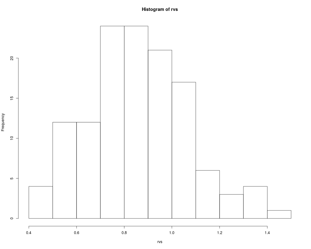
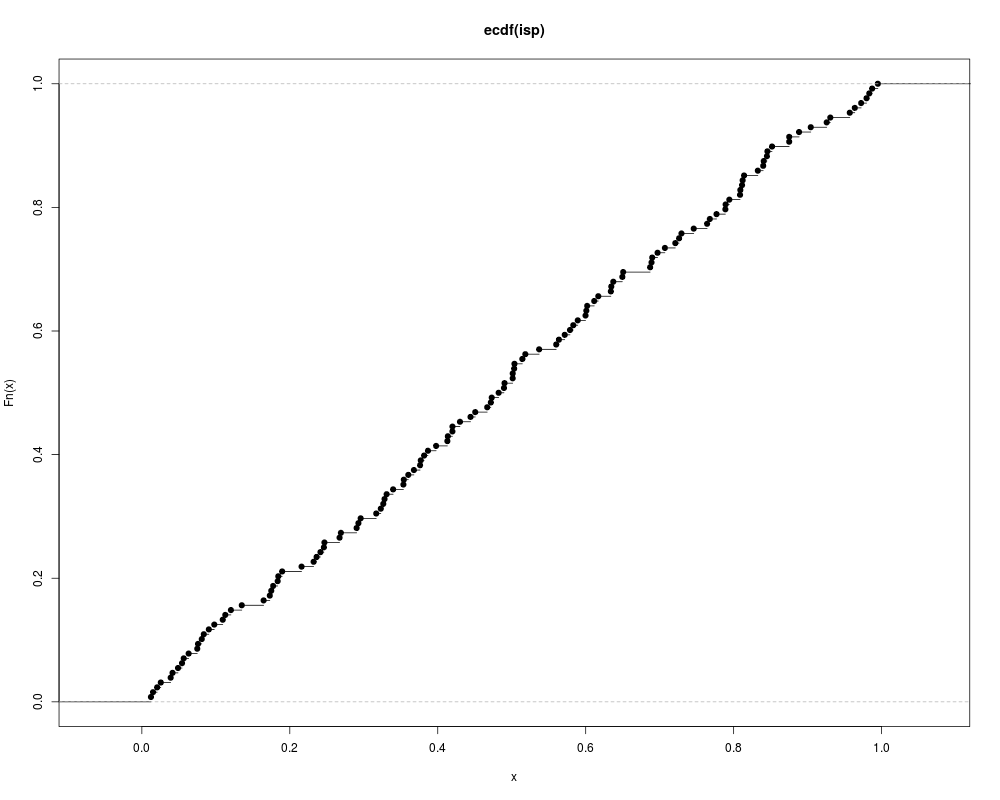
Examples

# generate some variates 
ngen <- 128
ope <- 253
df1 <- 8
df2 <- ope * 10
drag <- 0
# sample
rvs <- rsropt(ngen, df1, df2, drag, ope)
hist(rvs)
# these should be uniform:
isp <- psropt(rvs, df1, df2, drag, ope)
plot(ecdf(isp))

Results


R version 3.3.1 (2016-06-21) -- "Bug in Your Hair"
Copyright (C) 2016 The R Foundation for Statistical Computing
Platform: x86_64-pc-linux-gnu (64-bit)

R is free software and comes with ABSOLUTELY NO WARRANTY.
You are welcome to redistribute it under certain conditions.
Type 'license()' or 'licence()' for distribution details.

R is a collaborative project with many contributors.
Type 'contributors()' for more information and
'citation()' on how to cite R or R packages in publications.

Type 'demo()' for some demos, 'help()' for on-line help, or
'help.start()' for an HTML browser interface to help.
Type 'q()' to quit R.

> library(SharpeR)

Attaching package: 'SharpeR'

The following object is masked from 'package:base':

    summary

> png(filename="/home/ddbj/snapshot/RGM3/R_CC/result/SharpeR/dsropt.Rd_%03d_medium.png", width=480, height=480)
> ### Name: dsropt
> ### Title: The (non-central) maximal Sharpe ratio distribution.
> ### Aliases: dsropt psropt qsropt rsropt
> ### Keywords: distribution
> 
> ### ** Examples
> 
> # generate some variates 
> ngen <- 128
> ope <- 253
> df1 <- 8
> df2 <- ope * 10
> drag <- 0
> # sample
> rvs <- rsropt(ngen, df1, df2, drag, ope)
> hist(rvs)
> # these should be uniform:
> isp <- psropt(rvs, df1, df2, drag, ope)
> plot(ecdf(isp))
> 
> 
> 
> 
> 
> 
> dev.off()
null device 
          1 
>