The lambda-prime distribution.

Description

Distribution function and quantile function for LeCoutre's lambda-prime distribution with df degrees of freedom and the observed t-statistic, tstat.

Usage

plambdap(q, df, tstat, lower.tail = TRUE, log.p = FALSE)

qlambdap(p, df, tstat, lower.tail = TRUE, log.p = FALSE)

rlambdap(n, df, tstat)

Arguments

Details

Let t be distributed as a non-central t with v degrees of freedom and non-centrality parameter ncp. We can view this as

t = (Z + ncp)/sqrt(V/v)

where Z is a standard normal, ncp is the non-centrality parameter, V is a chi-square RV with v degrees of freedom, independent of Z. We can rewrite this as

ncp = t sqrt(V/v) + Z

Thus a 'lambda-prime' random variable with parameters t and v is one expressable as a sum

t sqrt(V/v) + Z

for Chi-square V with v d.f., independent from standard normal Z

Value

dlambdap gives the density, plambdap gives the distribution function, qlambdap gives the quantile function, and rlambdap generates random deviates.

Invalid arguments will result in return value NaN with a warning.

Note

plambdap should be an increasing function of the argument q, and decreasing in tstat. qlambdap should be increasing in p

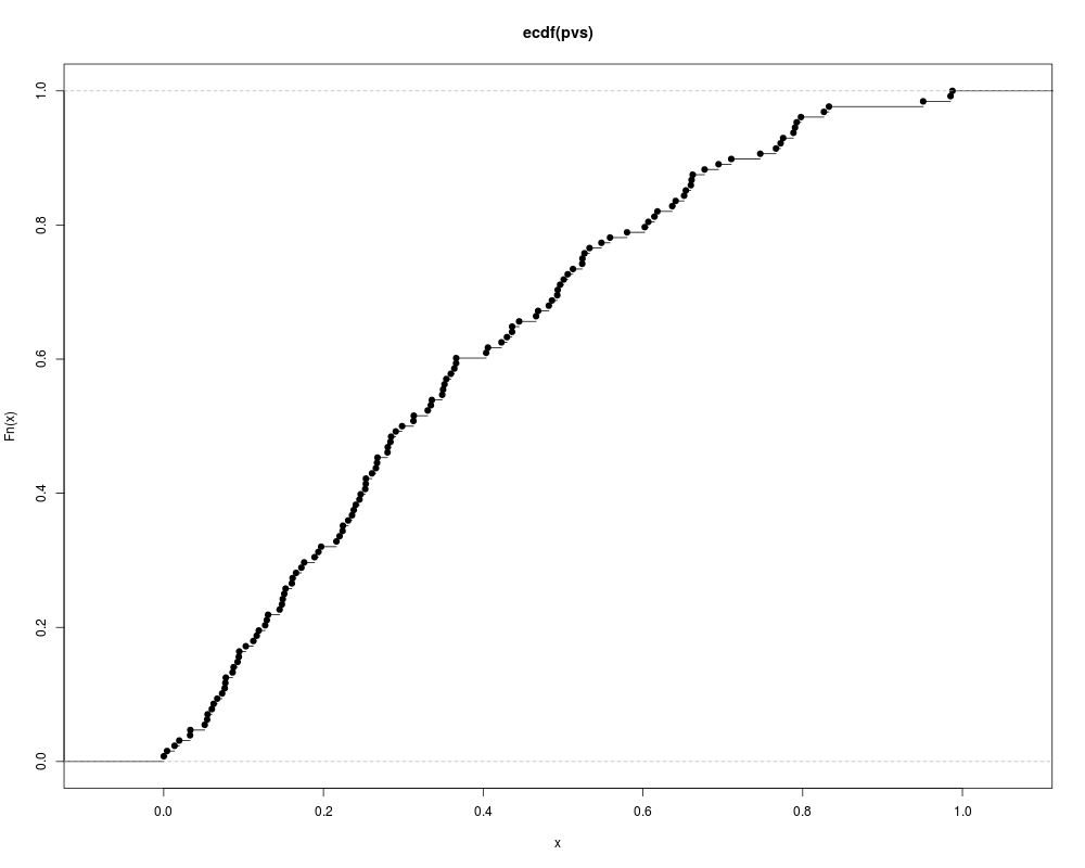
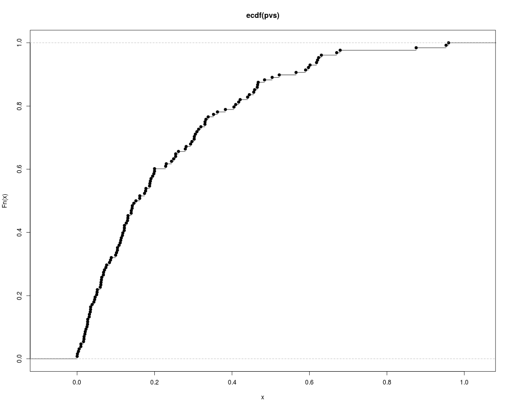
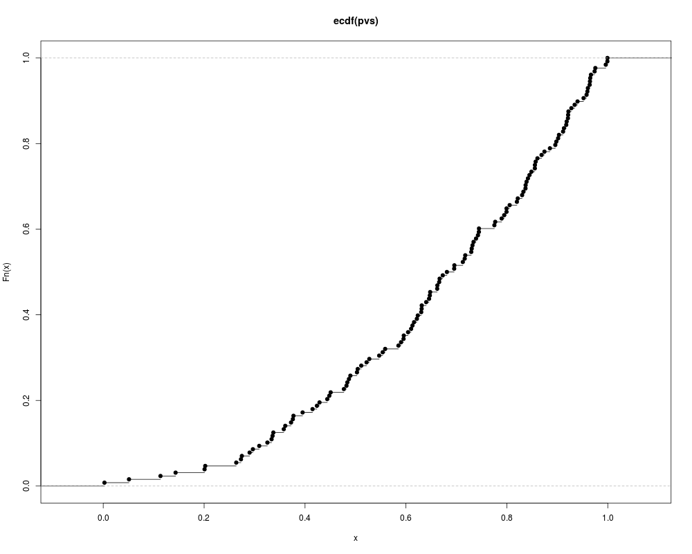
Author(s)

Steven E. Pav shabbychef@gmail.com

References

Lecoutre, Bruno. "Another look at confidence intervals for the noncentral t distribution." Journal of Modern Applied Statistical Methods 6, no. 1 (2007): 107–116. http://www.univ-rouen.fr/LMRS/Persopage/Lecoutre/telechargements/Lecoutre_Another_look-JMSAM2007_6(1).pdf

Lecoutre, Bruno. "Two useful distributions for Bayesian predictive procedures under normal models." Journal of Statistical Planning and Inference 79 (1999): 93–105.

See Also

t-distribution functions, dt,pt,qt,rt

Other sr: as.sr, confint.sr, dsr, is.sr, power.sr_test, predint, print.sr, reannualize, se, sr_equality_test, sr_test, sr_unpaired_test, sr_vcov, sr, summary

Examples

rvs <- rnorm(128)
pvs <- plambdap(rvs, 253*6, 0.5)
plot(ecdf(pvs))
pvs <- plambdap(rvs, 253*6, 1)
plot(ecdf(pvs))
pvs <- plambdap(rvs, 253*6, -0.5)
plot(ecdf(pvs))
# test vectorization:
qv <- qlambdap(0.1,128,2)
qv <- qlambdap(c(0.1),128,2)
qv <- qlambdap(c(0.2),128,2)
qv <- qlambdap(c(0.2),253,2)
qv <- qlambdap(c(0.1,0.2),128,2)
qv <- qlambdap(c(0.1,0.2),c(128,253),2)
qv <- qlambdap(c(0.1,0.2),c(128,253),c(2,4))
qv <- qlambdap(c(0.1,0.2),c(128,253),c(2,4,8,16))
# random generation
rv <- rlambdap(1000,252,2)

Results

R version 3.3.1 (2016-06-21) -- "Bug in Your Hair"
Copyright (C) 2016 The R Foundation for Statistical Computing
Platform: x86_64-pc-linux-gnu (64-bit)

R is free software and comes with ABSOLUTELY NO WARRANTY.
You are welcome to redistribute it under certain conditions.
Type 'license()' or 'licence()' for distribution details.

R is a collaborative project with many contributors.
Type 'contributors()' for more information and
'citation()' on how to cite R or R packages in publications.

Type 'demo()' for some demos, 'help()' for on-line help, or
'help.start()' for an HTML browser interface to help.
Type 'q()' to quit R.

> library(SharpeR)

Attaching package: 'SharpeR'

The following object is masked from 'package:base':

    summary

> png(filename="/home/ddbj/snapshot/RGM3/R_CC/result/SharpeR/plambdap.Rd_%03d_medium.png", width=480, height=480)
> ### Name: plambdap
> ### Title: The lambda-prime distribution.
> ### Aliases: plambdap qlambdap rlambdap
> ### Keywords: distribution
> 
> ### ** Examples
> 
> rvs <- rnorm(128)
> pvs <- plambdap(rvs, 253*6, 0.5)
> plot(ecdf(pvs))
> pvs <- plambdap(rvs, 253*6, 1)
> plot(ecdf(pvs))
> pvs <- plambdap(rvs, 253*6, -0.5)
> plot(ecdf(pvs))
> # test vectorization:
> qv <- qlambdap(0.1,128,2)
> qv <- qlambdap(c(0.1),128,2)
> qv <- qlambdap(c(0.2),128,2)
> qv <- qlambdap(c(0.2),253,2)
> qv <- qlambdap(c(0.1,0.2),128,2)
> qv <- qlambdap(c(0.1,0.2),c(128,253),2)
> qv <- qlambdap(c(0.1,0.2),c(128,253),c(2,4))
> qv <- qlambdap(c(0.1,0.2),c(128,253),c(2,4,8,16))
> # random generation
> rv <- rlambdap(1000,252,2)
> 
> 
> 
> 
> 
> 
> dev.off()
null device 
          1 
>