R Graphical Manual

Browse All

Last data update: 2014.03.03

R: Calculate SiZer Map

SiZer

R Documentation

Calculate SiZer Map

Description

Calculates the SiZer map from a given set of X and Y variables.

Usage

 SiZer(x, y, h=NA, x.grid=NA, degree=NA, derv=1, grid.length=41)

Arguments

`x`	data vector for the independent axis
`y`	data vector for the dependent axis
`h`	An integer representing how many bandwidths should be considered, or vector of length 2 representing the upper and lower limits h should take, or a vector of length greater than two indicating which bandwidths to examine.
`x.grid`	An integer representing how many bins to use along the x-axis, or a vector of length 2 representing the upper and lower limits the x-axis should take, or a vector of length greater than two indicating which x-values the derivative should be evaluated at.
`grid.length`	The default length of the `h.grid` or `x.grid` if the length of either is not given.
`derv`	The order of derivative for which to make the SiZer map.
`degree`	The degree of the local weighted polynomial used to smooth the data. This must be greater than or equal to `derv`.

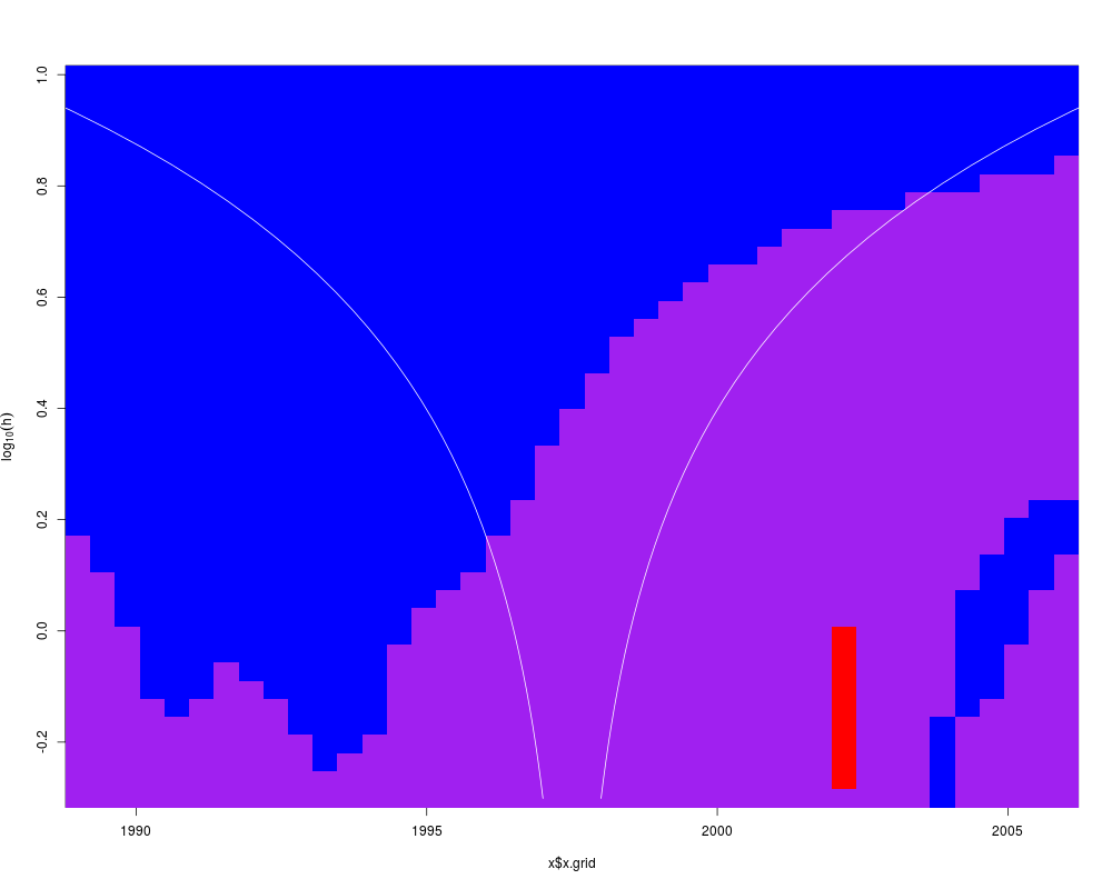
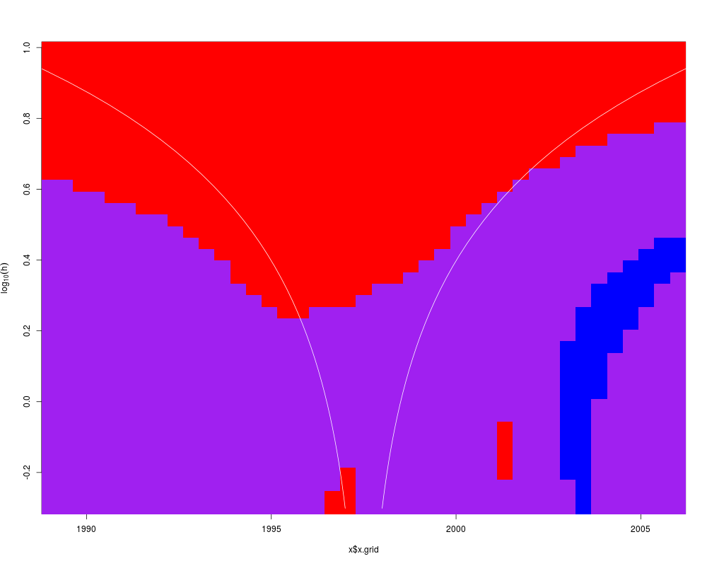
Details

SiZer stands for the Significant Zero crossings of the derivative. There are two dominate approaches in smoothing bivariate data: locally weighted regression or penalized splines. Both approaches require the use of a 'bandwidth' parameter that controls how much smoothing should be done. Unfortunately there is no uniformly best bandwidth selection procedure. SiZer (Chaudhuri and Marron, 1999) is a procedure that looks across a range of bandwidths and classifies the p-th derivative of the smoother into one of three states: significantly increasing (blue), possibly zero (purple), or significantly negative (red).

Value

Returns an SiZer object which has the following components:

`x.grid`	Vector of x-values at which the derivative was evaluated.
`h.grid`	Vector of bandwidth values for which a smoothing function was calculated.
`slopes`	Matrix of what category a particular x-value and bandwidth falls into (Increasing=1, Possibly Zero=0, Decreasing=-1, Not Enough Data=2).

Author(s)

Derek Sonderegger

References

Chaudhuri, P., and J. S. Marron. 1999. SiZer for exploration of structures in curves. Journal of the American Statistical Association 94:807-823.

Hannig, J., and J. S. Marron. 2006. Advanced distribution theory for SiZer. Journal of the American Statistical Association 101:484-499.

Sonderegger, D.L., Wang, H., Clements, W.H., and Noon, B.R. 2009. Using SiZer to detect thresholds in ecological data. Frontiers in Ecology and the Environment 7:190-195.

Examples

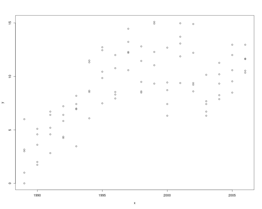
data('Arkansas')
x <- Arkansas$year
y <- Arkansas$sqrt.mayflies

plot(x,y)

# Calculate the SiZer map for the first derivative
SiZer.1 <- SiZer(x, y, h=c(.5,10), degree=1, derv=1)
plot(SiZer.1)

# Calculate the SiZer map for the second derivative
SiZer.2 <- SiZer(x, y, h=c(.5,10), degree=2, derv=2);
plot(SiZer.2)

# By setting the grid.length larger, we get a more detailed SiZer
# map but it takes longer to compute. 
#
# SiZer.3 <- SiZer(x, y, h=c(.5,10), grid.length=100, degree=1, derv=1)
# plot(SiZer.3)

Results


R version 3.3.1 (2016-06-21) -- "Bug in Your Hair"
Copyright (C) 2016 The R Foundation for Statistical Computing
Platform: x86_64-pc-linux-gnu (64-bit)

R is free software and comes with ABSOLUTELY NO WARRANTY.
You are welcome to redistribute it under certain conditions.
Type 'license()' or 'licence()' for distribution details.

R is a collaborative project with many contributors.
Type 'contributors()' for more information and
'citation()' on how to cite R or R packages in publications.

Type 'demo()' for some demos, 'help()' for on-line help, or
'help.start()' for an HTML browser interface to help.
Type 'q()' to quit R.

> library(SiZer)
Loading required package: splines
Loading required package: boot
> png(filename="/home/ddbj/snapshot/RGM3/R_CC/result/SiZer/SiZer.Rd_%03d_medium.png", width=480, height=480)
> ### Name: SiZer
> ### Title: Calculate SiZer Map
> ### Aliases: SiZer h.grid.create
> ### Keywords: hplot smooth
> 
> ### ** Examples
> 
> data('Arkansas')
> x <- Arkansas$year
> y <- Arkansas$sqrt.mayflies
> 
> plot(x,y)
> 
> # Calculate the SiZer map for the first derivative
> SiZer.1 <- SiZer(x, y, h=c(.5,10), degree=1, derv=1)
[1] 0.5
[1] 0.5388846
[1] 0.5807932
[1] 0.625961
[1] 0.6746414
[1] 0.7271077
[1] 0.7836543
[1] 0.8445984
[1] 0.9102821
[1] 0.981074
[1] 1.057371
[1] 1.139602
[1] 1.228228
[1] 1.323746
[1] 1.426693
[1] 1.537646
[1] 1.657227
[1] 1.786108
[1] 1.925012
[1] 2.074719
[1] 2.236068
[1] 2.409965
[1] 2.597386
[1] 2.799383
[1] 3.017088
[1] 3.251725
[1] 3.504608
[1] 3.777159
[1] 4.070905
[1] 4.387496
[1] 4.728708
[1] 5.096456
[1] 5.492803
[1] 5.919973
[1] 6.380365
[1] 6.87656
[1] 7.411344
[1] 7.987718
[1] 8.608917
[1] 9.278425
[1] 10
> plot(SiZer.1)
> 
> # Calculate the SiZer map for the second derivative
> SiZer.2 <- SiZer(x, y, h=c(.5,10), degree=2, derv=2);
[1] 0.5
[1] 0.5388846
[1] 0.5807932
[1] 0.625961
[1] 0.6746414
[1] 0.7271077
[1] 0.7836543
[1] 0.8445984
[1] 0.9102821
[1] 0.981074
[1] 1.057371
[1] 1.139602
[1] 1.228228
[1] 1.323746
[1] 1.426693
[1] 1.537646
[1] 1.657227
[1] 1.786108
[1] 1.925012
[1] 2.074719
[1] 2.236068
[1] 2.409965
[1] 2.597386
[1] 2.799383
[1] 3.017088
[1] 3.251725
[1] 3.504608
[1] 3.777159
[1] 4.070905
[1] 4.387496
[1] 4.728708
[1] 5.096456
[1] 5.492803
[1] 5.919973
[1] 6.380365
[1] 6.87656
[1] 7.411344
[1] 7.987718
[1] 8.608917
[1] 9.278425
[1] 10
> plot(SiZer.2)
> 
> # By setting the grid.length larger, we get a more detailed SiZer
> # map but it takes longer to compute. 
> #
> # SiZer.3 <- SiZer(x, y, h=c(.5,10), grid.length=100, degree=1, derv=1)
> # plot(SiZer.3)
> 
> 
> 
> 
> 
> dev.off()
null device 
          1 
>