R Graphical Manual

Browse All

Last data update: 2014.03.03

R: Locally-Weighted Polynomial Regression Smoother

locally.weighted.polynomial

R Documentation

Locally-Weighted Polynomial Regression Smoother

Description

Smoothes the given bivariate data using kernel regression.

Usage

locally.weighted.polynomial(x, y, h = NA, x.grid = NA, 
	degree = 1, kernel.type = "Normal")

Arguments

`x`	Vector of data for the independent variable
`y`	Vector of data for the dependent variable
`h`	The bandwidth for the kernel
`x.grid`	What x-values should the value of the smoother be calculated at.
`degree`	The degree of the polynomial to be fit at each x-value. The default is to fit a linear regression, ie degree=1.
`kernel.type`	What kernel to use. Valid choices are 'Normal', 'Epanechnikov', 'biweight', and 'triweight'

Details

The confidence intervals are created using the row-wise method of Hannig and Marron (2006).

Notice that the derivative to be estimated must be less than or equal to the degree of the polynomial initially fit to the data.

If the bandwidth is not given, the Sheather-Jones bandwidth selection method is used.

Value

Returns a LocallyWeightedPolynomial object that has the following elements:

`data`	A structure of the data used to generate the smoothing curve
`h`	The bandwidth used to generate the smoothing curve.
`x.grid`	The grid of x-values that we have estimated function value and derivative(s) for.
`degrees.freedom`	The effective sample size at each grid point
`Beta`	A matrix of estimated beta values. The number of rows is degrees+1, while the number of columns is the same as the length of x.grid. Notice that hat{f}(x_i) = β[1,i] hat{f'}(x_i) = β[2,i]1!* hat{f''}(x_i) = β[3,i]2!* and so on...
`Beta.var`	Matrix of estimated variances for `Beta`. Same structure as `Beta`.

Author(s)

Derek Sonderegger

References

Chaudhuri, P., and J. S. Marron. 1999. SiZer for exploration of structures in curves. Journal of the American Statistical Association 94 807-823.

Hannig, J., and J. S. Marron. 2006. Advanced distribution theory for SiZer. Journal of the American Statistical Association 101 484-499.

Sonderegger, D.L., Wang, H., Clements, W.H., and Noon, B.R. 2009. Using SiZer to detect thresholds in ecological data. Frontiers in Ecology and the Environment 7:190-195

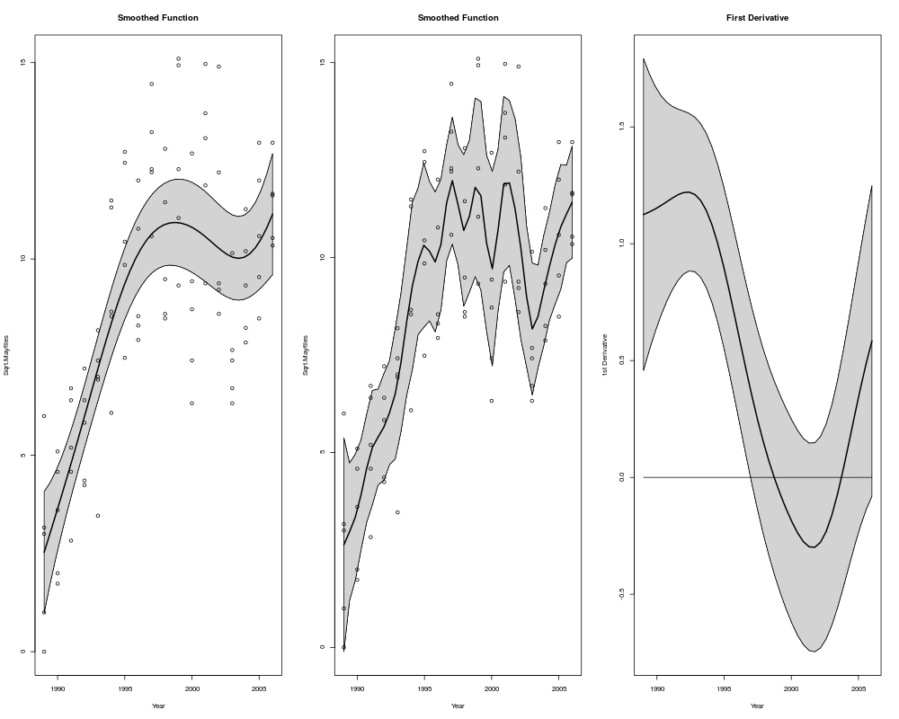
Examples

data(Arkansas)
x <- Arkansas$year
y <- Arkansas$sqrt.mayflies

layout(cbind(1,2,3))
model <- locally.weighted.polynomial(x,y)
plot(model, main='Smoothed Function', xlab='Year', ylab='Sqrt.Mayflies')

model2 <- locally.weighted.polynomial(x,y,h=.5)
plot(model2, main='Smoothed Function', xlab='Year', ylab='Sqrt.Mayflies')

model3 <- locally.weighted.polynomial(x,y, degree=1)
plot(model3, derv=1, main='First Derivative', xlab='Year', ylab='1st Derivative')

Results


R version 3.3.1 (2016-06-21) -- "Bug in Your Hair"
Copyright (C) 2016 The R Foundation for Statistical Computing
Platform: x86_64-pc-linux-gnu (64-bit)

R is free software and comes with ABSOLUTELY NO WARRANTY.
You are welcome to redistribute it under certain conditions.
Type 'license()' or 'licence()' for distribution details.

R is a collaborative project with many contributors.
Type 'contributors()' for more information and
'citation()' on how to cite R or R packages in publications.

Type 'demo()' for some demos, 'help()' for on-line help, or
'help.start()' for an HTML browser interface to help.
Type 'q()' to quit R.

> library(SiZer)
Loading required package: splines
Loading required package: boot
> png(filename="/home/ddbj/snapshot/RGM3/R_CC/result/SiZer/locally.weighted.polynomial.Rd_%03d_medium.png", width=480, height=480)
> ### Name: locally.weighted.polynomial
> ### Title: Locally-Weighted Polynomial Regression Smoother
> ### Aliases: locally.weighted.polynomial calc.CI.LocallyWeightedPolynomial
> ###   find.state find.state.changes find.states kernel.h positive.part
> ###   x.grid.create
> ### Keywords: smooth
> 
> ### ** Examples
> 
> data(Arkansas)
> x <- Arkansas$year
> y <- Arkansas$sqrt.mayflies
> 
> layout(cbind(1,2,3))
> model <- locally.weighted.polynomial(x,y)
> plot(model, main='Smoothed Function', xlab='Year', ylab='Sqrt.Mayflies')
> 
> model2 <- locally.weighted.polynomial(x,y,h=.5)
> plot(model2, main='Smoothed Function', xlab='Year', ylab='Sqrt.Mayflies')
> 
> model3 <- locally.weighted.polynomial(x,y, degree=1)
> plot(model3, derv=1, main='First Derivative', xlab='Year', ylab='1st Derivative')
> 
> 
> 
> 
> 
> dev.off()
null device 
          1 
>