R Graphical Manual

Browse All

Last data update: 2014.03.03

R: Plot a LocallyWeightedPolynomial object

plot.LocallyWeightedPolynomial

R Documentation

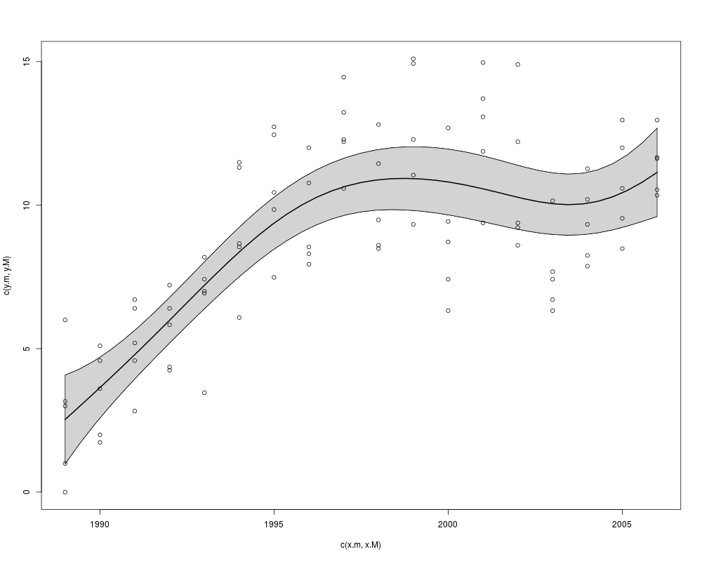
Plot a LocallyWeightedPolynomial object

Description

Creates a plot of an object created by locally.weighted.polynomial.

Usage

## S3 method for class 'LocallyWeightedPolynomial'
plot(x, derv = 0, CI.method = 2, 
	alpha = 0.05, use.ess = TRUE, draw.points = TRUE, ...)

Arguments

`x`	LocallyWeightedPolynomial object
`derv`	Derivative to be plotted. Default is 0 - which plots the smoothed function.
`CI.method`	What method should be used to calculate the confidence interval about the estimated line. The methods are from Hannig and Marron (2006), where 1 is the point-wise estimate, and 2 is the row-wise estimate.
`alpha`	The CI has a 1-alpha/2 level of significance.
`use.ess`	ESS stands for the estimated sample size. If at any point along the x-axis, the ESS is too small, then we will not plot unless use.ess=FALSE.
`draw.points`	Should the data points be included in the graph?
`...`	Additional arguments to be passed to the graphing functions.

Author(s)

Derek Sonderegger

References

Hannig, J., and J. S. Marron. 2006. Advanced distribution theory for SiZer. Journal of the American Statistical Association 101:484-499.

Sonderegger, D.L., Wang, H., Clements, W.H., and Noon, B.R. 2009. Using SiZer to detect thresholds in ecological data. Frontiers in Ecology and the Environment 7:190-195.

Examples

data('Arkansas')
x <- Arkansas$year
y <- Arkansas$sqrt.mayflies

model <- locally.weighted.polynomial(x,y)
plot(model)

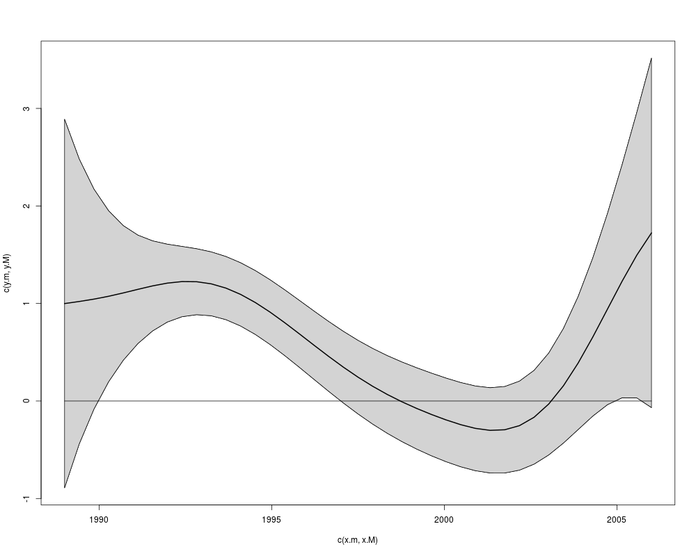
model <- locally.weighted.polynomial(x,y,degree=2)
plot(model, derv=1)
plot(model, derv=2)

Results


R version 3.3.1 (2016-06-21) -- "Bug in Your Hair"
Copyright (C) 2016 The R Foundation for Statistical Computing
Platform: x86_64-pc-linux-gnu (64-bit)

R is free software and comes with ABSOLUTELY NO WARRANTY.
You are welcome to redistribute it under certain conditions.
Type 'license()' or 'licence()' for distribution details.

R is a collaborative project with many contributors.
Type 'contributors()' for more information and
'citation()' on how to cite R or R packages in publications.

Type 'demo()' for some demos, 'help()' for on-line help, or
'help.start()' for an HTML browser interface to help.
Type 'q()' to quit R.

> library(SiZer)
Loading required package: splines
Loading required package: boot
> png(filename="/home/ddbj/snapshot/RGM3/R_CC/result/SiZer/plot.LocallyWeightedPolynomial.Rd_%03d_medium.png", width=480, height=480)
> ### Name: plot.LocallyWeightedPolynomial
> ### Title: Plot a LocallyWeightedPolynomial object
> ### Aliases: plot.LocallyWeightedPolynomial
> ### Keywords: hplot
> 
> ### ** Examples
> 
> data('Arkansas')
> x <- Arkansas$year
> y <- Arkansas$sqrt.mayflies
> 
> model <- locally.weighted.polynomial(x,y)
> plot(model)
> 
> model <- locally.weighted.polynomial(x,y,degree=2)
> plot(model, derv=1)
> plot(model, derv=2)
> 
> 
> 
> 
> 
> dev.off()
null device 
          1 
>