R Graphical Manual

Browse All

Last data update: 2014.03.03

R: First Passage Time in 1-Dim SDE

fptsde1d

R Documentation

First Passage Time in 1-Dim SDE

Description

The (S3) generic function fptsde1d for simulate first-passage-time (f.p.t) in 1-dim stochastic differential equations.

Usage

fptsde1d(N, ...)
## Default S3 method:
fptsde1d(N = 1000, M = 100, x0 = 0, t0 = 0, T = 1, Dt, 
   boundary, drift, diffusion, alpha = 0.5, mu = 0.5, 
   type = c("ito", "str"), method = c("euler", "milstein", "predcorr", 
   "smilstein", "taylor", "heun", "rk1", "rk2", "rk3"), ...)
						  
						  
## S3 method for class 'fptsde1d'
summary(object, ...)
## S3 method for class 'fptsde1d'
mean(x, ...)
## S3 method for class 'fptsde1d'
median(x, ...)
## S3 method for class 'fptsde1d'
quantile(x, ...)
## S3 method for class 'fptsde1d'
kurtosis(x, ...)
## S3 method for class 'fptsde1d'
skewness(x, ...)
## S3 method for class 'fptsde1d'
moment(x, order = 2, ...)
## S3 method for class 'fptsde1d'
bconfint(x, level=0.95, ...)
## S3 method for class 'fptsde1d'
plot(x, ...)

Arguments

`N`	size of sde.
`M`	size of fpt.
`x0`	initial value of the process at time `t0`.
`t0`	initial time.
`T`	final time.
`Dt`	time step of the simulation (discretization). If it is `missing` a default Dt = (T-t0)/N.
`boundary`	an `expression` of a constant or time-dependent boundary.
`drift`	drift coefficient: an `expression` of two variables `t` and `x`.
`diffusion`	diffusion coefficient: an `expression` of two variables `t` and `x`.
`alpha, mu`	weight of the predictor-corrector scheme; the default `alpha = 0.5` and `mu = 0.5`.
`type`	sde of the type Ito or Stratonovich.
`method`	numerical methods of simulation, the default `method = "euler"`; see `snssde1d`.
`x, object`	an object inheriting from class `"fptsde1d"`.
`order`	order of moment.
`level`	the confidence level required.
`...`	further arguments for (non-default) methods.

Details

The function fptsde1d returns a random variable tau(X(t),S(t)) "first passage time", is defined as :

tau(X(t),S(t))={t>=0; X(t) >= S(t)}, if X(t0) < S(t0)

tau(X(t),S(t))={t>=0; X(t) <= S(t)}, if X(t0) > S(t0)

with S(t) is through a continuous boundary (barrier).

Value

fptsde1d returns an object inheriting from class "fptsde1d".

fpt

numeric vector of fpt (first passage time).

Author(s)

A.C. Guidoum, K. Boukhetala.

References

Argyrakisa, P. and G.H. Weiss (2006). A first-passage time problem for many random walkers. Physica A. 363, 343–347.

Aytug H., G. J. Koehler (2000). New stopping criterion for genetic algorithms. European Journal of Operational Research, 126, 662–674.

Boukhetala, K. (1996) Modelling and simulation of a dispersion pollutant with attractive centre. ed by Computational Mechanics Publications, Southampton ,U.K and Computational Mechanics Inc, Boston, USA, 245–252.

Boukhetala, K. (1998a). Estimation of the first passage time distribution for a simulated diffusion process. Maghreb Math.Rev, 7(1), 1–25.

Boukhetala, K. (1998b). Kernel density of the exit time in a simulated diffusion. les Annales Maghrebines De L ingenieur, 12, 587–589.

Ding, M. and G. Rangarajan. (2004). First Passage Time Problem: A Fokker-Planck Approach. New Directions in Statistical Physics. ed by L. T. Wille. Springer. 31–46.

Roman, R.P., Serrano, J. J., Torres, F. (2008). First-passage-time location function: Application to determine first-passage-time densities in diffusion processes. Computational Statistics and Data Analysis. 52, 4132–4146.

Roman, R.P., Serrano, J. J., Torres, F. (2012). An R package for an efficient approximation of first-passage-time densities for diffusion processes based on the FPTL function. Applied Mathematics and Computation, 218, 8408–8428.

Gardiner, C. W. (1997). Handbook of Stochastic Methods. Springer-Verlag, New York.

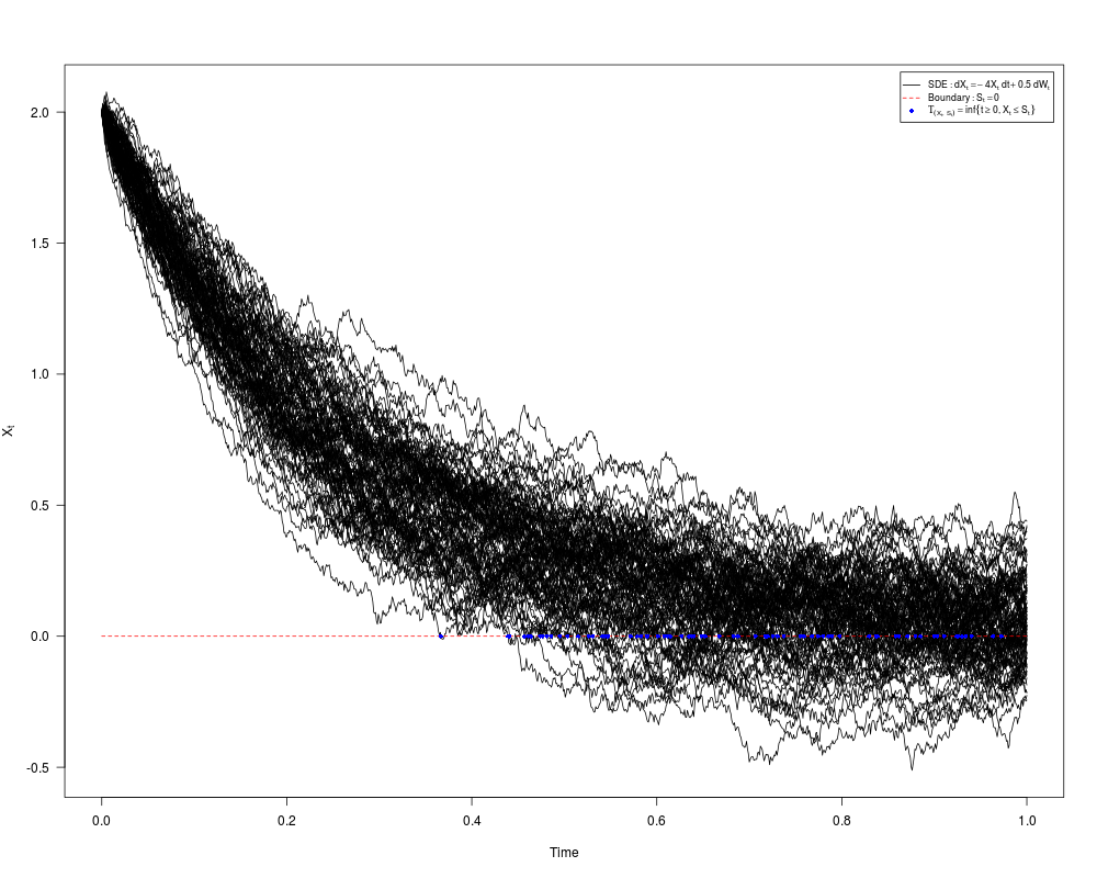
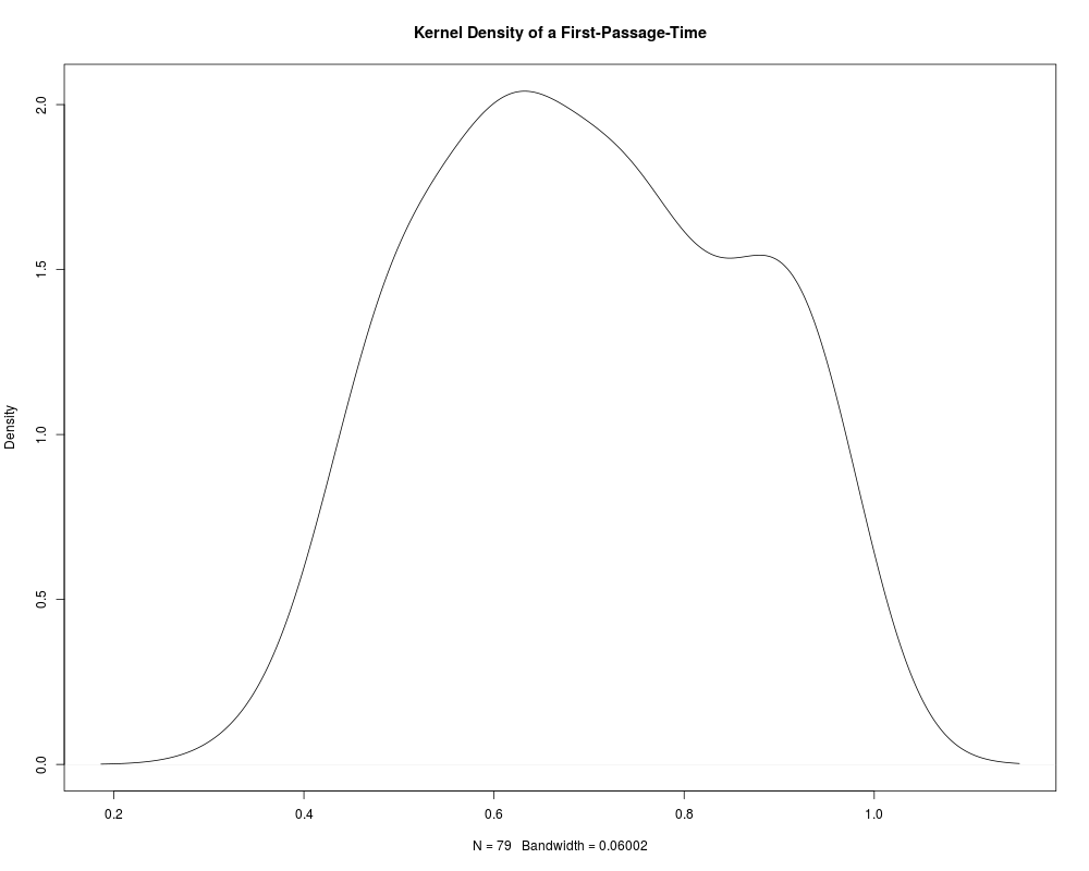
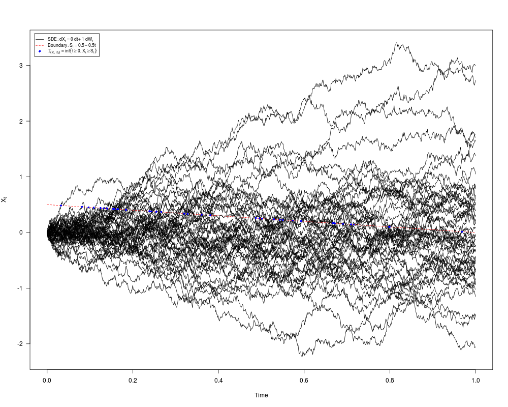
Examples


## Example 1: Ito SDE
## dX(t) = -4*X(t) *dt + 0.5*dW(t)
## S(t) = 0 (constant boundary)
set.seed(1234)

f <- expression( -4*x )
g <- expression( 0.5 )
St <- expression(0) 
res1 <- fptsde1d(drift=f,diffusion=g,boundary=St,x0=2)
res1
plot(res1)
summary(res1)
plot(density(res1$fpt[!is.na(res1$fpt)]),main="Kernel Density of a First-Passage-Time")

## Example 2: Ito SDE
## X(t) Brownian motion
## S(t) = 0.3+0.2*t (time-dependent boundary)
set.seed(1234)

f <- expression( 0 )
g <- expression( 1 )
St <- expression(0.5-0.5*t) 
res2 <- fptsde1d(drift=f,diffusion=g,boundary=St,M=50)
res2
summary(res2)
plot(res2,pos=3)
dev.new()
plot(density(res2$fpt[!is.na(res2$fpt)]),main="Kernel Density of a First-Passage-Time")

## Example 3: Stratonovich SDE
## dX(t) = 0.5*X(t)*t *dt + sqrt(1+X(t)^2) o dW(t)
## S(t) = -0.5*sqrt(t) + exp(t^2) (time-dependent boundary)
set.seed(1234)

f <- expression( 0.5*x*t )
g <- expression( sqrt(1+x^2) )
St <- expression(-0.5*sqrt(t)+exp(t^2))
res3 <- fptsde1d(drift=f,diffusion=g,boundary=St,x0=2,M=50,type="srt")
res3
summary(res3)
plot(res3,legend=FALSE)
dev.new()
plot(density(res3$fpt[!is.na(res3$fpt)]),main="Kernel Density of a First-Passage-Time")

Results


R version 3.3.1 (2016-06-21) -- "Bug in Your Hair"
Copyright (C) 2016 The R Foundation for Statistical Computing
Platform: x86_64-pc-linux-gnu (64-bit)

R is free software and comes with ABSOLUTELY NO WARRANTY.
You are welcome to redistribute it under certain conditions.
Type 'license()' or 'licence()' for distribution details.

R is a collaborative project with many contributors.
Type 'contributors()' for more information and
'citation()' on how to cite R or R packages in publications.

Type 'demo()' for some demos, 'help()' for on-line help, or
'help.start()' for an HTML browser interface to help.
Type 'q()' to quit R.

> library(Sim.DiffProc)
Package 'Sim.DiffProc' version 3.2 loaded.
help(Sim.DiffProc) for summary information.
> png(filename="/home/ddbj/snapshot/RGM3/R_CC/result/Sim.DiffProc/fptsde1d.Rd_%03d_medium.png", width=480, height=480)
> ### Name: fptsde1d
> ### Title: First Passage Time in 1-Dim SDE
> ### Aliases: fptsde1d fptsde1d.default summary.fptsde1d mean.fptsde1d
> ###   median.fptsde1d quantile.fptsde1d kurtosis.fptsde1d skewness.fptsde1d
> ###   moment.fptsde1d bconfint.fptsde1d plot.fptsde1d
> ### Keywords: fpt sde ts
> 
> ### ** Examples
> 
> 
> ## Example 1: Ito SDE
> ## dX(t) = -4*X(t) *dt + 0.5*dW(t)
> ## S(t) = 0 (constant boundary)
> set.seed(1234)
> 
> f <- expression( -4*x )
> g <- expression( 0.5 )
> St <- expression(0) 
> res1 <- fptsde1d(drift=f,diffusion=g,boundary=St,x0=2)
> res1
$SDE
Ito Sde 1D:
	| dX(t) = -4 * X(t) * dt + 0.5 * dW(t)
Method:
	| Euler scheme of order 0.5
Summary:
	| Size of process	| N  = 1000.
	| Number of simulation	| M  = 100.
	| Initial value		| x0 = 2.
	| Time of process	| t in [0,1].
	| Discretization	| Dt = 0.001.

$boundary
[1] 0

$fpt
  [1] 0.5445283 0.9242204 0.7555601        NA 0.4951891        NA 0.6524345
  [8] 0.5893863        NA 0.9633318 0.6832877        NA 0.7745919 0.6268057
 [15] 0.7856547 0.5265549 0.8367654 0.8849836        NA 0.7256442 0.8795968
 [22] 0.6879598 0.7894158 0.4568457        NA 0.3666177 0.6347135 0.4859602
 [29]        NA        NA 0.8585762        NA        NA 0.5306337 0.5412482
 [36] 0.4738468 0.6145441 0.9106270 0.6012699 0.8708522 0.5149896 0.6373736
 [43] 0.9725667 0.6349144 0.6485953 0.8294137 0.7975120        NA 0.6676193
 [50] 0.5789512 0.8385933 0.9639104 0.4409355        NA 0.8613485        NA
 [57] 0.7067830 0.4814192 0.5472524        NA 0.4614059 0.5827597 0.9299972
 [64] 0.9403937 0.7306951 0.7591328        NA        NA 0.4639474 0.6120858
 [71]        NA 0.9030982 0.9338551 0.6079475 0.5716893 0.9260307 0.6401436
 [78]        NA        NA 0.7180299 0.7184662 0.4766718 0.7176569 0.9263782
 [85]        NA 0.7184844 0.5458184 0.7797918 0.6487542 0.6271423 0.7373581
 [92] 0.5034689 0.5902315        NA 0.4392058 0.7199643 0.8996260 0.9336041
 [99] 0.7678059 0.7853798

attr(,"class")
[1] "fptsde1d"
> plot(res1)
> summary(res1)

	 Monte-Carlo Statistics for the F.P.T of X(t)
| T(S,X) = inf{t >= 0 : X(t) <= 0}
                       fpt(x)
NA's                       21
Mean                 0.695074
Variance             0.025534
Median               0.687960
First quartile       0.575320
Third quartile       0.833090
Skewness             0.056140
Kurtosis             1.879444
Moment of order 2    0.025211
Moment of order 3    0.000229
Moment of order 4    0.001225
Moment of order 5    0.000005
Bound conf Inf (95%) 0.440849
Bound conf Sup (95%) 0.963361
> plot(density(res1$fpt[!is.na(res1$fpt)]),main="Kernel Density of a First-Passage-Time")
> 
> ## Example 2: Ito SDE
> ## X(t) Brownian motion
> ## S(t) = 0.3+0.2*t (time-dependent boundary)
> set.seed(1234)
> 
> f <- expression( 0 )
> g <- expression( 1 )
> St <- expression(0.5-0.5*t) 
> res2 <- fptsde1d(drift=f,diffusion=g,boundary=St,M=50)
> res2
$SDE
Ito Sde 1D:
	| dX(t) = 0 * dt + 1 * dW(t)
Method:
	| Euler scheme of order 0.5
Summary:
	| Size of process	| N  = 1000.
	| Number of simulation	| M  = 50.
	| Initial value		| x0 = 0.
	| Time of process	| t in [0,1].
	| Discretization	| Dt = 0.001.

$boundary
0.5 - 0.5 * t

$fpt
 [1] 0.18427791 0.31967753         NA         NA 0.16349454 0.24337756
 [7] 0.79935044         NA 0.13985877 0.52955992 0.32077610 0.10897391
[13] 0.12463495 0.25503695 0.09665703 0.66682298 0.16580403 0.15417660
[19] 0.71582317 0.48730562         NA         NA 0.70962364 0.23883215
[25] 0.38105403         NA 0.69082941         NA 0.54320229 0.96865422
[31] 0.55016194 0.59280188 0.36067354         NA 0.57290741 0.13227151
[37] 0.67164184 0.32817041 0.18356179         NA 0.08105678 0.26624097
[43] 0.15572302         NA         NA 0.49530753 0.03233182 0.79837152
[49] 0.50160495 0.15697774

attr(,"class")
[1] "fptsde1d"
> summary(res2)

	 Monte-Carlo Statistics for the F.P.T of X(t)
| T(S,X) = inf{t >= 0 : X(t) >= 0.5 - 0.5 * t}
                       fpt(x)
NA's                       11
Mean                 0.381734
Variance             0.061289
Median               0.320776
First quartile       0.160236
Third quartile       0.561535
Skewness             0.489324
Kurtosis             2.015688
Moment of order 2    0.059717
Moment of order 3    0.007425
Moment of order 4    0.007572
Moment of order 5    0.002389
Bound conf Inf (95%) 0.078621
Bound conf Sup (95%) 0.807816
> plot(res2,pos=3)
> dev.new()
Error in dev.new() : no suitable unused file name for pdf()
Execution halted