R Graphical Manual

Browse All

Last data update: 2014.03.03

R: First Passage Time in 2-Dim SDE

fptsde2d

R Documentation

First Passage Time in 2-Dim SDE

Description

The (S3) generic function fptsde2d for simulate first-passage-time (f.p.t) in 2-dim stochastic differential equations.

Usage

fptsde2d(N, ...)
## Default S3 method:
fptsde2d(N = 1000, M = 100, x0 = 0, y0 = 0, t0 = 0, T = 1, Dt, 
   boundary, driftx, diffx, drifty, diffy, alpha = 0.5, mu = 0.5, type = 
   c("ito", "str"), method = c("euler", "milstein", "predcorr", "smilstein", 
   "taylor", "heun", "rk1", "rk2", "rk3"), ...)		

   
## S3 method for class 'fptsde2d'
summary(object, ...)	
## S3 method for class 'fptsde2d'
mean(x, ...)
## S3 method for class 'fptsde2d'
median(x, ...)
## S3 method for class 'fptsde2d'
quantile(x, ...)
## S3 method for class 'fptsde2d'
kurtosis(x, ...)
## S3 method for class 'fptsde2d'
skewness(x, ...)
## S3 method for class 'fptsde2d'
moment(x, order = 2, ...)
## S3 method for class 'fptsde2d'
bconfint(x, level=0.95, ...)
## S3 method for class 'fptsde2d'
plot(x, ...)

Arguments

`N`	size of sde.
`M`	size of fpt.
`x0, y0`	initial value of the process X(t) and Y(t) at time `t0`.
`t0`	initial time.
`T`	final time.
`Dt`	time step of the simulation (discretization). If it is `missing` a default Dt = (T-t0)/N.
`boundary`	an `expression` of a constant or time-dependent boundary.
`driftx, drifty`	drift coefficient: an `expression` of three variables `t`, `x` and `y` for process X(t) and Y(t).
`diffx, diffy`	diffusion coefficient: an `expression` of three variables `t`, `x` and `y` for process X(t) and Y(t).
`alpha, mu`	weight of the predictor-corrector scheme; the default `alpha = 0.5` and `mu = 0.5`.
`type`	sde of the type Ito or Stratonovich.
`method`	numerical methods of simulation, the default `method = "euler"`; see `snssde2d`.
`x, object`	an object inheriting from class `"fptsde2d"`.
`order`	order of moment.
`level`	the confidence level required.
`...`	further arguments for (non-default) methods.

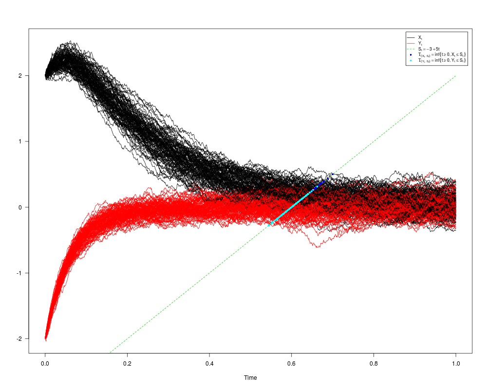
Details

The function fptsde1d returns a random variable (tau(X(t),S(t)),tau(Y(t),S(t))) "first passage time", is defined as :

tau(X(t),S(t))={t>=0; X(t) >= S(t)}, if X(t0) < S(t0)

tau(Y(t),S(t))={t>=0; Y(t) >= S(t)}, if Y(t0) < S(t0)

and:

tau(X(t),S(t))={t>=0; X(t) <= S(t)}, if X(t0) > S(t0)

tau(Y(t),S(t))={t>=0; Y(t) <= S(t)}, if Y(t0) > S(t0)

with S(t) is through a continuous boundary (barrier).

Value

fptsde2d returns an object inheriting from class "fptsde2d".

fptx, fpty

a vector of couple 'fpt' (tau(X(t),S(t)),tau(Y(t),S(t))).

Author(s)

A.C. Guidoum, K. Boukhetala.

References

Argyrakisa, P. and G.H. Weiss (2006). A first-passage time problem for many random walkers. Physica A. 363, 343–347.

Aytug H., G. J. Koehler (2000). New stopping criterion for genetic algorithms. European Journal of Operational Research, 126, 662–674.

Boukhetala, K. (1996) Modelling and simulation of a dispersion pollutant with attractive centre. ed by Computational Mechanics Publications, Southampton ,U.K and Computational Mechanics Inc, Boston, USA, 245–252.

Boukhetala, K. (1998a). Estimation of the first passage time distribution for a simulated diffusion process. Maghreb Math.Rev, 7(1), 1–25.

Boukhetala, K. (1998b). Kernel density of the exit time in a simulated diffusion. les Annales Maghrebines De L ingenieur, 12, 587–589.

Ding, M. and G. Rangarajan. (2004). First Passage Time Problem: A Fokker-Planck Approach. New Directions in Statistical Physics. ed by L. T. Wille. Springer. 31–46.

Roman, R.P., Serrano, J. J., Torres, F. (2008). First-passage-time location function: Application to determine first-passage-time densities in diffusion processes. Computational Statistics and Data Analysis. 52, 4132–4146.

Roman, R.P., Serrano, J. J., Torres, F. (2012). An R package for an efficient approximation of first-passage-time densities for diffusion processes based on the FPTL function. Applied Mathematics and Computation, 218, 8408–8428.

Gardiner, C. W. (1997). Handbook of Stochastic Methods. Springer-Verlag, New York.

Examples


## dX(t) = 5*(-1-Y(t))*X(t) * dt + 0.5 * dW1(t)          
## dY(t) = 5*(-1-X(t))*Y(t) * dt + 0.5 * dW2(t)
## x0 = 2, y0 = -2, and barrier -3+5*t.
## W1(t) and W2(t) two independent Brownian motion
set.seed(1234)

fx <- expression(5*(-1-y)*x)
gx <- expression(0.5)
fy <- expression(5*(-1-x)*y)
gy <- expression(0.5)

St <- expression(-3+5*t)

res <- fptsde2d(driftx=fx,diffx=gx,drifty=fy,diffy=gy,boundary=St,
                x0=2,y0=-2)
res
summary(res)
plot(res)
##

fptx <- res$fptx
fpty <- res$fpty
X1 <- cbind(fptx,fpty)
## library(sm)
## sm.density(X1,display="persp")

Results


R version 3.3.1 (2016-06-21) -- "Bug in Your Hair"
Copyright (C) 2016 The R Foundation for Statistical Computing
Platform: x86_64-pc-linux-gnu (64-bit)

R is free software and comes with ABSOLUTELY NO WARRANTY.
You are welcome to redistribute it under certain conditions.
Type 'license()' or 'licence()' for distribution details.

R is a collaborative project with many contributors.
Type 'contributors()' for more information and
'citation()' on how to cite R or R packages in publications.

Type 'demo()' for some demos, 'help()' for on-line help, or
'help.start()' for an HTML browser interface to help.
Type 'q()' to quit R.

> library(Sim.DiffProc)
Package 'Sim.DiffProc' version 3.2 loaded.
help(Sim.DiffProc) for summary information.
> png(filename="/home/ddbj/snapshot/RGM3/R_CC/result/Sim.DiffProc/fptsde2d.Rd_%03d_medium.png", width=480, height=480)
> ### Name: fptsde2d
> ### Title: First Passage Time in 2-Dim SDE
> ### Aliases: fptsde2d fptsde2d.default summary.fptsde2d mean.fptsde2d
> ###   median.fptsde2d quantile.fptsde2d kurtosis.fptsde2d skewness.fptsde2d
> ###   moment.fptsde2d bconfint.fptsde2d plot.fptsde2d
> ### Keywords: fpt sde ts mts
> 
> ### ** Examples
> 
> 
> ## dX(t) = 5*(-1-Y(t))*X(t) * dt + 0.5 * dW1(t)          
> ## dY(t) = 5*(-1-X(t))*Y(t) * dt + 0.5 * dW2(t)
> ## x0 = 2, y0 = -2, and barrier -3+5*t.
> ## W1(t) and W2(t) two independent Brownian motion
> set.seed(1234)
> 
> fx <- expression(5*(-1-y)*x)
> gx <- expression(0.5)
> fy <- expression(5*(-1-x)*y)
> gy <- expression(0.5)
> 
> St <- expression(-3+5*t)
> 
> res <- fptsde2d(driftx=fx,diffx=gx,drifty=fy,diffy=gy,boundary=St,
+                 x0=2,y0=-2)
> res
$SDE
Ito Sde 2D:
	| dX(t) = 5 * (-1 - Y(t)) * X(t) * dt + 0.5 * dW1(t)
	| dY(t) = 5 * (-1 - X(t)) * Y(t) * dt + 0.5 * dW2(t)
Method:
	| Euler scheme of order 0.5
Summary:
	| Size of process	| N  = 1000.
	| Number of simulation	| M  = 100.
	| Initial values	| (x0,y0) = (2,-2).
	| Time of process	| t in [0,1].
	| Discretization	| Dt = 0.001.

$boundary
-3 + 5 * t

$fptx
  [1] 0.6047413 0.6240573 0.6495478 0.6497464 0.6246658 0.6537598 0.6680226
  [8] 0.5996549 0.6434420 0.6334217 0.6229044 0.6049682 0.6272445 0.6009809
 [15] 0.6659500 0.6245398 0.6504229 0.5661780 0.6622888 0.6792500 0.6123626
 [22] 0.6165871 0.6329416 0.6341970 0.6328549 0.6443622 0.6175694 0.6579726
 [29] 0.6604464 0.6349960 0.6005590 0.6518056 0.6192896 0.6997678 0.6639580
 [36] 0.6262199 0.6479090 0.6215602 0.6361245 0.6215246 0.6366694 0.5912661
 [43] 0.6703629 0.6177974 0.6252187 0.5979482 0.6466468 0.6499089 0.6153245
 [50] 0.6327192 0.6190643 0.6198844 0.6226452 0.5921108 0.6457871 0.6228074
 [57] 0.6875926 0.5915456 0.6543998 0.6600266 0.6535355 0.6406480 0.6511594
 [64] 0.6522912 0.6779212 0.5865785 0.6554440 0.6328378 0.6293758 0.5961436
 [71] 0.6305228 0.6292932 0.6109144 0.6216743 0.5987734 0.6223292 0.6219099
 [78] 0.6190965 0.6339259 0.5919647 0.6612402 0.6471265 0.6390919 0.6478464
 [85] 0.6590154 0.6224804 0.6627242 0.6376235 0.6371600 0.6415000 0.6345309
 [92] 0.6083908 0.6468429 0.6705290 0.6768190 0.6087074 0.6172294 0.6075580
 [99] 0.6423921 0.6724459

$fpty
  [1] 0.6194456 0.5669556 0.5690901 0.6128980 0.6072852 0.6065007 0.6091704
  [8] 0.5877053 0.5713714 0.6061686 0.6065655 0.5918935 0.5907941 0.6485664
 [15] 0.5935385 0.5859929 0.5669673 0.5691950 0.5788887 0.5835343 0.5750274
 [22] 0.6340122 0.6193305 0.6169691 0.5700007 0.6313327 0.5750525 0.5953716
 [29] 0.5964311 0.6037166 0.5704867 0.6117621 0.5851602 0.5756763 0.5826980
 [36] 0.6051136 0.5727720 0.6625831 0.6169102 0.5856820 0.5661684 0.5749829
 [43] 0.5446837 0.5917209 0.6041700 0.5595606 0.6350452 0.5867976 0.5923071
 [50] 0.6055162 0.5987023 0.6525159 0.6149906 0.6372166 0.6144033 0.5836673
 [57] 0.5512619 0.6134058 0.5724796 0.5662623 0.5607117 0.6191409 0.6213329
 [64] 0.6278571 0.6245903 0.6263856 0.6274735 0.6108360 0.6182089 0.5831149
 [71] 0.6394778 0.6403859 0.5958757 0.6042229 0.5702555 0.6136525 0.5749452
 [78] 0.6015048 0.6026376 0.6043788 0.6029009 0.5709548 0.5772711 0.6168131
 [85] 0.5827607 0.5543004 0.5789899 0.6070445 0.5699023 0.5967427 0.5972329
 [92] 0.5883591 0.5580396 0.6237154 0.5791152 0.6062854 0.6443307 0.5629168
 [99] 0.5802551 0.5590110

attr(,"class")
[1] "fptsde2d"
> summary(res)

	 Monte-Carlo Statistics for the F.P.T of (X(t),Y(t))
| T(S,X) = inf{t >=  0  : X(t) <=  -3 + 5 * t }
| T(S,Y) = inf{t >=  0  : Y(t) <=  -3 + 5 * t }

                       fpt(x)   fpt(y)
NA's                        0        0
Mean                 0.633861 0.596484
Variance             0.000610 0.000630
Median               0.633182 0.596153
First quartile       0.619088 0.575046
Third quartile       0.650607 0.613840
Skewness             0.018118 0.275919
Kurtosis             2.805812 2.429327
Moment of order 2    0.000604 0.000624
Moment of order 3    0.000000 0.000004
Moment of order 4    0.000001 0.000001
Moment of order 5    0.000000 0.000000
Bound conf Inf (95%) 0.591399 0.556077
Bound conf Sup (95%) 0.678619 0.646554
> plot(res)
> ##
> 
> fptx <- res$fptx
> fpty <- res$fpty
> X1 <- cbind(fptx,fpty)
> ## library(sm)
> ## sm.density(X1,display="persp")
> 
> 
> 
> 
> 
> dev.off()
null device 
          1 
>