R Graphical Manual

Browse All

Last data update: 2014.03.03

R: Random Number Generators for 1-Dim SDE

rsde1d

R Documentation

Random Number Generators for 1-Dim SDE

Description

The (S3) generic function rsde1d for simulate random number generators to generate 1-dim sde.

Usage

rsde1d(N, ...)
## Default S3 method:
rsde1d(N = 1000, M = 100, x0 = 0, t0 = 0, T = 1, Dt, tau = 0.5, 
   drift, diffusion, alpha = 0.5, mu = 0.5,type = c("ito", "str"), 
   method = c("euler", "milstein", "predcorr", "smilstein", "taylor",
   "heun", "rk1", "rk2", "rk3"), ...)
   
## S3 method for class 'rsde1d'
summary(object, ...)
## S3 method for class 'rsde1d'
mean(x, ...)
## S3 method for class 'rsde1d'
median(x, ...)
## S3 method for class 'rsde1d'
quantile(x, ...)
## S3 method for class 'rsde1d'
kurtosis(x, ...)
## S3 method for class 'rsde1d'
skewness(x, ...)
## S3 method for class 'rsde1d'
moment(x, order = 2, ...)
## S3 method for class 'rsde1d'
bconfint(x, level=0.95, ...)
## S3 method for class 'rsde1d'
plot(x, ...)

Arguments

`N`	size of sde.
`M`	number of random numbers to be geneated.
`x0`	initial value of the process at time `t0`.
`t0`	initial time.
`T`	final time.
`Dt`	time step of the simulation (discretization). If it is `missing` a default Dt = (T-t0)/N.
`tau`	moment (time) between `t0` and `T`. Random number generated at `time=tau`.
`drift`	drift coefficient: an `expression` of two variables `t` and `x`.
`diffusion`	diffusion coefficient: an `expression` of two variables `t` and `x`.
`alpha, mu`	weight of the predictor-corrector scheme; the default `alpha = 0.5` and `mu = 0.5`.
`type`	sde of the type Ito or Stratonovich.
`method`	numerical methods of simulation, the default `method = "euler"`; see `snssde1d`.
`x, object`	an object inheriting from class `"rsde1d"`.
`order`	order of moment.
`level`	the confidence level required.
`...`	further arguments for (non-default) methods.

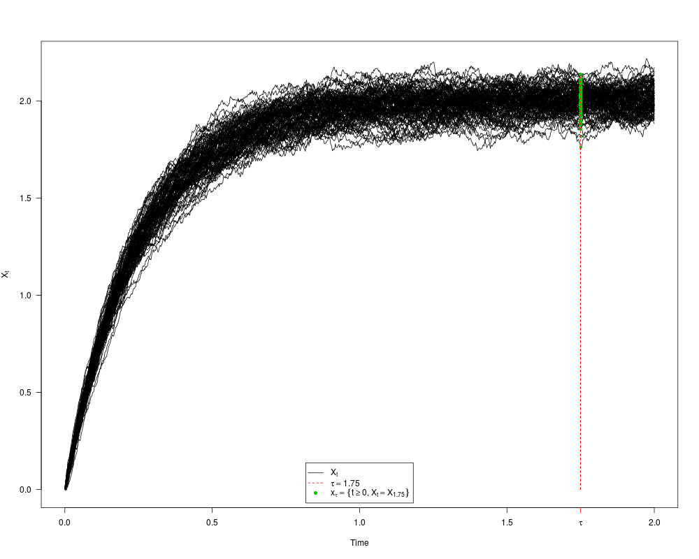
Details

The function rsde1d returns a random variable x(tau) realize at time t=tau defined by :

x(tau) = { t>=0 ; x = X(tau) }

with tau is a fixed time between t0 and T.

Value

rsde1d returns an object inheriting from class "rsde1d".

`x`	a vector of random numbers of 1-dim sde realize at time t=tau.

Author(s)

A.C. Guidoum, K. Boukhetala.

Examples


## Example 1: Ito sde
## dX(t) = 2*(3-X(t)) *dt + dW(t)
set.seed(1234)

f <- expression( 4*(2-x) )
g <- expression( 0.2 )
res <- rsde1d(drift=f,diffusion=g,tau=1.75,T=2)
res
summary(res)
plot(res,pos=7,cex=1)
dev.new()
plot(density(res$x))

## Example 2: Stratonovich sde
## dX(t) = (-2*(X(t)<=0)+2*(X(t)>=0)) *dt + 0.5 o dW(t)
set.seed(1234)

f <- expression(-2*(x<=0)+2*(x>=0))
g <- expression(0.5)
res1 <- rsde1d(drift=f,diffusion=g,tau=0.95123,type="str")
res1
summary(res1)
plot(res1,pos=3,cex=1)
dev.new()
plot(density(res1$x))

Results


R version 3.3.1 (2016-06-21) -- "Bug in Your Hair"
Copyright (C) 2016 The R Foundation for Statistical Computing
Platform: x86_64-pc-linux-gnu (64-bit)

R is free software and comes with ABSOLUTELY NO WARRANTY.
You are welcome to redistribute it under certain conditions.
Type 'license()' or 'licence()' for distribution details.

R is a collaborative project with many contributors.
Type 'contributors()' for more information and
'citation()' on how to cite R or R packages in publications.

Type 'demo()' for some demos, 'help()' for on-line help, or
'help.start()' for an HTML browser interface to help.
Type 'q()' to quit R.

> library(Sim.DiffProc)
Package 'Sim.DiffProc' version 3.2 loaded.
help(Sim.DiffProc) for summary information.
> png(filename="/home/ddbj/snapshot/RGM3/R_CC/result/Sim.DiffProc/rsde1d.Rd_%03d_medium.png", width=480, height=480)
> ### Name: rsde1d
> ### Title: Random Number Generators for 1-Dim SDE
> ### Aliases: rsde1d rsde1d.default summary.rsde1d mean.rsde1d median.rsde1d
> ###   quantile.rsde1d kurtosis.rsde1d skewness.rsde1d moment.rsde1d
> ###   bconfint.rsde1d plot.rsde1d
> ### Keywords: sde ts mts random generators
> 
> ### ** Examples
> 
> 
> ## Example 1: Ito sde
> ## dX(t) = 2*(3-X(t)) *dt + dW(t)
> set.seed(1234)
> 
> f <- expression( 4*(2-x) )
> g <- expression( 0.2 )
> res <- rsde1d(drift=f,diffusion=g,tau=1.75,T=2)
> res
$SDE
Ito Sde 1D:
	| dX(t) = 4 * (2 - X(t)) * dt + 0.2 * dW(t)
Method:
	| Euler scheme of order 0.5
Summary:
	| Size of process	| N  = 1000.
	| Number of simulation	| M  = 100.
	| Initial value		| x0 = 0.
	| Time of process	| t in [0,2].
	| Discretization	| Dt = 0.002.

$tau
[1] 1.75

$x
  [1] 2.072283 2.062621 1.986077 2.077760 2.037233 2.010189 2.033496 2.064015
  [9] 2.104233 2.038959 2.047938 2.093251 2.013670 1.967484 1.939248 2.000085
 [17] 1.998211 1.976267 2.136915 1.919043 1.958735 1.884107 1.928722 2.041939
 [25] 2.067877 1.993190 1.760132 2.078408 2.065617 2.115602 1.928742 2.089686
 [33] 2.018324 1.974549 2.012332 1.962306 2.113016 2.025422 1.965744 1.940587
 [41] 2.001910 1.966100 2.018273 2.024002 1.944715 1.898817 1.874669 2.037483
 [49] 2.028293 1.976268 1.970138 2.019775 2.049845 2.021422 1.959783 2.097288
 [57] 2.027670 1.939661 1.892079 2.041701 1.890057 1.931804 2.001186 1.963521
 [65] 1.997631 1.818307 2.076412 2.021954 2.001780 2.060242 2.116575 2.059347
 [73] 2.026378 2.077149 1.953372 2.011269 2.091266 1.988934 2.030704 1.962506
 [81] 2.035795 1.960059 1.987517 2.032664 2.114291 2.015030 2.062932 2.057662
 [89] 2.038180 1.854728 2.015134 1.986510 2.004736 2.026931 2.029292 1.922127
 [97] 1.978073 2.029185 1.977688 1.902891

attr(,"class")
[1] "rsde1d"
> summary(res)

	Monte-Carlo Statistics for X(t) at t = 1.75
                             x
Mean                  2.004057
Variance              0.004523
Median                2.014350
First quartile        1.965188
Third quartile        2.043439
Skewness             -0.715679
Kurtosis              3.949483
Moment of order 2     0.004478
Moment of order 3    -0.000218
Moment of order 4     0.000081
Moment of order 5    -0.000011
Bound conf Inf (95%)  1.864200
Bound conf Sup (95%)  2.114979
> plot(res,pos=7,cex=1)
> dev.new()
Error in dev.new() : no suitable unused file name for pdf()
Execution halted