R Graphical Manual

Browse All

Last data update: 2014.03.03

R: Random Number Generators for 2-Dim SDE

rsde2d

R Documentation

Random Number Generators for 2-Dim SDE

Description

The (S3) generic function rsde2d for simulate random number generators to generate 2-dim sde.

Usage

rsde2d(N, ...)
## Default S3 method:
rsde2d(N = 1000, M = 100, x0 = 0, y0 = 0, t0 = 0, T = 1, Dt, tau = 0.5, 
   driftx, diffx, drifty, diffy, alpha = 0.5, mu = 0.5, type = c("ito", "str"), 
   method = c("euler", "milstein", "predcorr", "smilstein", "taylor", 
   "heun", "rk1", "rk2", "rk3"), ...)				 
   
   
## S3 method for class 'rsde2d'
summary(object, ...)
## S3 method for class 'rsde2d'
mean(x, ...)
## S3 method for class 'rsde2d'
median(x, ...)
## S3 method for class 'rsde2d'
quantile(x, ...)
## S3 method for class 'rsde2d'
kurtosis(x, ...)
## S3 method for class 'rsde2d'
skewness(x, ...)
## S3 method for class 'rsde2d'
moment(x, order = 2, ...)
## S3 method for class 'rsde2d'
bconfint(x, level=0.95, ...)
## S3 method for class 'rsde2d'
plot(x, ...)

Arguments

`N`	size of sde.
`M`	number of random numbers to be geneated.
`x0, y0`	initial value of the process X(t) and Y(t) at time `t0`.
`t0`	initial time.
`T`	final time.
`Dt`	time step of the simulation (discretization). If it is `missing` a default Dt = (T-t0)/N.
`tau`	moment (time) between `t0` and `T`. Random number generated at `time=tau`.
`driftx, drifty`	drift coefficient: an `expression` of three variables `t`, `x` and `y` for process X(t) and Y(t).
`diffx, diffy`	diffusion coefficient: an `expression` of three variables `t`, `x` and `y` for process X(t) and Y(t).
`alpha, mu`	weight of the predictor-corrector scheme; the default `alpha = 0.5` and `mu = 0.5`.
`type`	sde of the type Ito or Stratonovich.
`method`	numerical methods of simulation, the default `method = "euler"`; see `snssde2d`.
`x, object`	an object inheriting from class `"rsde2d"`.
`order`	order of moment.
`level`	the confidence level required.
`...`	further arguments for (non-default) methods.

Details

The function rsde2d returns a two random variables (x(tau),y(tau)) realize at time t=tau defined by :

x(tau)={t>=0; x = X(tau)}

y(tau)={t>=0; y = Y(tau)}

with tau is a fixed time between t0 and T.

Value

rsde2d returns an object inheriting from class "rsde2d".

x, y

a vector of random numbers of 2-dim sde realize at time time t=tau, the couple (x(tau),y(tau)).

Author(s)

A.C. Guidoum, K. Boukhetala.

Examples


## Example 1:
## random numbers of two standard Brownian motion W1(t) and W2(t) at time = 1
set.seed(1234)

fx <- expression(0)
gx <- expression(1)
fy <- expression(0)
gy <- expression(1)
res1 <- rsde2d(driftx=fx,diffx=gx,drifty=fy,diffy=gy,tau=1)
res1
summary(res1)
X <- cbind(res1$x,res1$y)
## library(sm)
## sm.density(X,display="persp")

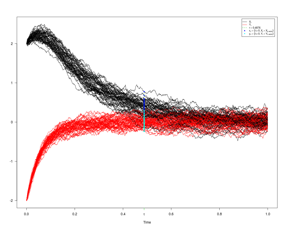
## Example 2: 
## dX(t) = 5*(-1-Y(t))*X(t) * dt + 0.5 * dW1(t)          
## dY(t) = 5*(-1-X(t))*Y(t) * dt + 0.5 * dW2(t)
## W1(t) and W2(t) two independent Brownian motion
set.seed(1234)

fx <- expression(5*(-1-y)*x)
gx <- expression(0.5)
fy <- expression(5*(-1-x)*y)
gy <- expression(0.5)
res2 <- rsde2d(driftx=fx,diffx=gx,drifty=fy,diffy=gy,tau=0.4876
               ,x0=2,y0=-2,M=50)
res2
summary(res2)
plot(res2,union=TRUE)
dev.new()
plot(res2,union=FALSE)
X <- cbind(res2$x,res2$y)
## sm.density(X,display="persp")

Results


R version 3.3.1 (2016-06-21) -- "Bug in Your Hair"
Copyright (C) 2016 The R Foundation for Statistical Computing
Platform: x86_64-pc-linux-gnu (64-bit)

R is free software and comes with ABSOLUTELY NO WARRANTY.
You are welcome to redistribute it under certain conditions.
Type 'license()' or 'licence()' for distribution details.

R is a collaborative project with many contributors.
Type 'contributors()' for more information and
'citation()' on how to cite R or R packages in publications.

Type 'demo()' for some demos, 'help()' for on-line help, or
'help.start()' for an HTML browser interface to help.
Type 'q()' to quit R.

> library(Sim.DiffProc)
Package 'Sim.DiffProc' version 3.2 loaded.
help(Sim.DiffProc) for summary information.
> png(filename="/home/ddbj/snapshot/RGM3/R_CC/result/Sim.DiffProc/rsde2d.Rd_%03d_medium.png", width=480, height=480)
> ### Name: rsde2d
> ### Title: Random Number Generators for 2-Dim SDE
> ### Aliases: rsde2d rsde2d.default summary.rsde2d mean.rsde2d median.rsde2d
> ###   quantile.rsde2d kurtosis.rsde2d skewness.rsde2d moment.rsde2d
> ###   bconfint.rsde2d plot.rsde2d
> ### Keywords: sde ts mts random generators
> 
> ### ** Examples
> 
> 
> ## Example 1:
> ## random numbers of two standard Brownian motion W1(t) and W2(t) at time = 1
> set.seed(1234)
> 
> fx <- expression(0)
> gx <- expression(1)
> fy <- expression(0)
> gy <- expression(1)
> res1 <- rsde2d(driftx=fx,diffx=gx,drifty=fy,diffy=gy,tau=1)
> res1
$SDE
Ito Sde 2D:
	| dX(t) = 0 * dt + 1 * dW1(t)
	| dY(t) = 0 * dt + 1 * dW2(t)
Method:
	| Euler scheme of order 0.5
Summary:
	| Size of process	| N  = 1000.
	| Number of simulation	| M  = 100.
	| Initial values	| (x0,y0) = (0,0).
	| Time of process	| t in [0,1].
	| Discretization	| Dt = 0.001.

$tau
[1] 1

$x
  [1] -0.752480843  1.702508137 -0.886742315  1.102104818 -0.072030515
  [6]  0.690516597  1.250107590  0.336372924  1.890800159  0.109238964
 [11]  0.099397754 -0.637768773 -1.347715323 -2.440436791  0.909373295
 [16]  0.836954108  0.526877871  0.284616553  2.733666268  1.192575060
 [21] -1.665951693 -1.324730493 -0.365312965  0.006597265  0.904601706
 [26]  0.402344080 -0.951783158  0.607011758  0.577166109 -1.688961042
 [31] -1.217521278  1.871545948 -0.521119439  1.325818238  0.285569020
 [36]  0.421780885  1.994326282 -1.050162417  0.552445149  0.206196169
 [41] -1.070028554 -0.315776716  0.756446587 -0.369655616  0.629929557
 [46] -0.311790467 -0.857326695 -0.570031127  0.192493894 -1.039283215
 [51]  0.544427675 -0.528700758 -0.810824784 -1.347182044  0.466129652
 [56]  0.528125966  1.773809511 -0.463832732  0.432883872  1.442536907
 [61]  0.910333558 -0.421111647  0.434936145  1.468225095  0.554064864
 [66] -0.061054415  0.354880902 -0.255413407  0.544084923 -0.744957932
 [71]  0.446529741  2.333070081 -1.029377983  0.121452880 -0.114991379
 [76]  0.503900038  1.098777909 -0.530587598 -0.024000252 -0.608981619
 [81]  0.140523756  0.499919675  1.572362867  2.356740424 -0.235453842
 [86]  0.177443346  0.414325908 -0.883922171 -0.319481616  0.167257016
 [91]  0.255289435 -0.336055142  1.469777758  0.429926441  0.122399389
 [96]  0.819122320  0.295999038 -0.949693068 -0.491286273  2.152657224

$y
  [1]  0.50667148 -0.96360037 -0.32068759 -1.02845604  0.11419805  0.79195738
  [7]  0.80923953  0.84248818 -0.34221365  0.43938815  0.36861426 -0.49791714
 [13] -1.58097598 -1.41807390 -0.09193726  1.50024399 -0.91115708 -0.19324185
 [19]  1.26212073 -1.12776770  0.26550537  0.75268083 -0.73995138  1.28352488
 [25] -0.29790765  0.66369237 -0.08150428 -0.02660853 -1.60906884  0.89637653
 [31]  0.20016235 -0.01808949 -0.21559015  0.74908918 -0.59886326 -0.03648556
 [37] -0.82987985  1.64760794  1.01975432  0.33085089 -2.30629103  1.13496302
 [43] -1.06537708 -0.27594047 -1.07943124 -0.29387762  2.01770803  0.53843675
 [49]  0.73067729  0.50170097 -0.20272859  0.74783627  1.22412106  0.88100868
 [55]  1.37145009 -0.42355719 -0.74806384 -0.68381214  0.24044379 -0.98884966
 [61] -1.27127987 -0.66405976 -0.14360769  0.02681467  0.56160040  1.58960893
 [67] -0.30683514 -0.57384290 -0.33813803 -0.04289656  0.16139669  0.04550287
 [73] -0.12226641 -0.91142192 -0.71865725 -0.08089410  1.24669966  0.10357728
 [79] -0.64647203  0.07614455 -0.72978126  0.12103374  0.32459263  1.57242143
 [85] -0.31042552 -1.73227711  0.13327040 -0.29184858  0.87328694 -1.12755055
 [91] -1.24015472  0.68576181 -0.21097617  1.09578779  0.22431963 -0.29951479
 [97]  0.59530819 -0.79143416 -0.69461776  0.76865006

attr(,"class")
[1] "rsde2d"
> summary(res1)

    Monte-Carlo Statistics for X(t) and Y(t) at t = 1

                             x         y
Mean                  0.196178 -0.002086
Variance              0.959849  0.724598
Median                0.230743 -0.039691
First quartile       -0.498745 -0.650869
Third quartile        0.645076  0.669210
Skewness              0.166416 -0.012700
Kurtosis              2.942410  2.620024
Moment of order 2     0.950251  0.717352
Moment of order 3     0.156495 -0.007833
Moment of order 4     2.710874  1.375625
Moment of order 5     0.800026 -0.258054
Bound conf Inf (95%) -1.514789 -1.595725
Bound conf Sup (95%)  2.247374  1.581445
> X <- cbind(res1$x,res1$y)
> ## library(sm)
> ## sm.density(X,display="persp")
> 
> ## Example 2: 
> ## dX(t) = 5*(-1-Y(t))*X(t) * dt + 0.5 * dW1(t)          
> ## dY(t) = 5*(-1-X(t))*Y(t) * dt + 0.5 * dW2(t)
> ## W1(t) and W2(t) two independent Brownian motion
> set.seed(1234)
> 
> fx <- expression(5*(-1-y)*x)
> gx <- expression(0.5)
> fy <- expression(5*(-1-x)*y)
> gy <- expression(0.5)
> res2 <- rsde2d(driftx=fx,diffx=gx,drifty=fy,diffy=gy,tau=0.4876
+                ,x0=2,y0=-2,M=50)
> res2
$SDE
Ito Sde 2D:
	| dX(t) = 5 * (-1 - Y(t)) * X(t) * dt + 0.5 * dW1(t)
	| dY(t) = 5 * (-1 - X(t)) * Y(t) * dt + 0.5 * dW2(t)
Method:
	| Euler scheme of order 0.5
Summary:
	| Size of process	| N  = 1000.
	| Number of simulation	| M  = 50.
	| Initial values	| (x0,y0) = (2,-2).
	| Time of process	| t in [0,1].
	| Discretization	| Dt = 0.001.

$tau
[1] 0.4876

$x
 [1]  0.37045552  0.52300479  0.08369982  0.28796583  0.25915916  0.23919130
 [7]  0.34059663  0.77575169  0.32267635  0.50306037  0.59706326  0.57773318
[13]  0.54614539  0.59442533  0.18566895  0.40655062  0.41854655  0.24183743
[19]  0.56001159  0.25042614  0.14825070  0.54434343  0.31354847  0.53183272
[25]  0.37875266  0.15298765  0.09969632  0.48721758  0.38654370  0.18791596
[31] -0.07168162  0.22393001  0.42480426  0.33881001  0.16476811  0.19151850
[37]  0.67748695  0.16934174  0.47200220  0.39271166  0.44638779  0.25307664
[43]  0.27497295  0.45441872  0.49790286  0.41883353  0.45537985 -0.13282119
[49]  0.21242166  0.46013589

$y
 [1]  0.08576661 -0.07231530 -0.07169320 -0.04497045  0.22615801 -0.06443680
 [7] -0.10454925 -0.11699850  0.08153500 -0.12291282 -0.09796212 -0.10531677
[13]  0.03880450 -0.14027926  0.07586430  0.12449890 -0.03415597 -0.15423662
[19] -0.05868709  0.11265533  0.12442072  0.05346850 -0.02095579  0.05879950
[25] -0.17410546  0.15276767  0.03557542  0.04474690 -0.23673402  0.05061763
[31] -0.01266982  0.29053100  0.21046903 -0.01561020 -0.04888774  0.05779271
[37]  0.03093737  0.03127232  0.05133502  0.01186592 -0.18423635  0.17584998
[43] -0.08324319 -0.03013000 -0.07323272 -0.22485228 -0.05276285  0.27190322
[49]  0.15889527 -0.06292103

attr(,"class")
[1] "rsde2d"
> summary(res2)

    Monte-Carlo Statistics for X(t) and Y(t) at t = 0.4876

                             x         y
Mean                  0.352789  0.002954
Variance              0.033810  0.015042
Median                0.374604 -0.014140
First quartile        0.227745 -0.073003
Third quartile        0.483414  0.071598
Skewness             -0.260806  0.301220
Kurtosis              2.935137  2.601741
Moment of order 2     0.033133  0.014741
Moment of order 3    -0.001621  0.000556
Moment of order 4     0.003355  0.000589
Moment of order 5    -0.000479  0.000053
Bound conf Inf (95%) -0.036721 -0.215714
Bound conf Sup (95%)  0.659392  0.261611
> plot(res2,union=TRUE)
> dev.new()
Error in dev.new() : no suitable unused file name for pdf()
Execution halted