R Graphical Manual

Browse All

Last data update: 2014.03.03

R: Random Number Generators for 3-Dim SDE

rsde3d

R Documentation

Random Number Generators for 3-Dim SDE

Description

The (S3) generic function rsde3d for simulate random number generators to generate 3-dim sde.

Usage

rsde3d(N, ...)
## Default S3 method:
rsde3d(N = 1000, M = 100, x0 = 0, y0 = 0, z0 = 0, t0 = 0, T = 1, Dt, tau = 0.5,
   driftx, diffx, drifty, diffy, driftz, diffz, alpha = 0.5, mu = 0.5, 
   type = c("ito", "str"), method = c("euler", "milstein", "predcorr",
   "smilstein", "taylor", "heun", "rk1", "rk2", "rk3"), ...)		

   
## S3 method for class 'rsde3d'
summary(object, ...)
## S3 method for class 'rsde3d'
mean(x, ...)
## S3 method for class 'rsde3d'
median(x, ...)
## S3 method for class 'rsde3d'
quantile(x, ...)
## S3 method for class 'rsde3d'
kurtosis(x, ...)
## S3 method for class 'rsde3d'
skewness(x, ...)
## S3 method for class 'rsde3d'
moment(x, order = 2, ...)
## S3 method for class 'rsde3d'
bconfint(x, level=0.95, ...)
## S3 method for class 'rsde3d'
plot(x, ...)

Arguments

`N`	size of sde.
`M`	number of random numbers to be geneated.
`x0, y0, z0`	initial value of the process X(t), Y(t) and Z(t) at time `t0`.
`t0`	initial time.
`T`	final time.
`Dt`	time step of the simulation (discretization). If it is `missing` a default Dt = (T-t0)/N.
`tau`	moment (time) between `t0` and `T`. Random number generated at `time=tau`.
`driftx, drifty, driftz`	drift coefficient: an `expression` of four variables `t`, `x`, `y` and `z` for process X(t), Y(t) and Z(t).
`diffx, diffy, diffz`	diffusion coefficient: an `expression` of four variables `t`, `x`, `y` and `z` for process X(t), Y(t) and Z(t).
`alpha, mu`	weight of the predictor-corrector scheme; the default `alpha = 0.5` and `mu = 0.5`.
`type`	sde of the type Ito or Stratonovich.
`method`	numerical methods of simulation, the default `method = "euler"`; see `snssde3d`.
`x, object`	an object inheriting from class `"rsde2d"`.
`order`	order of moment.
`level`	the confidence level required.
`...`	further arguments for (non-default) methods.

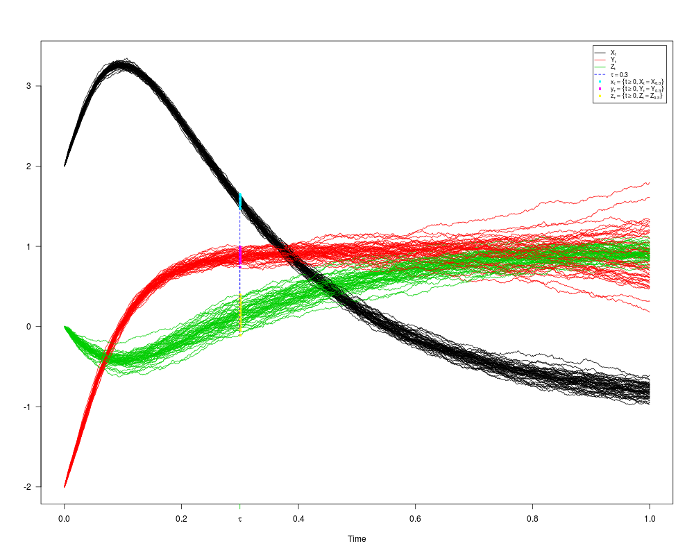
Details

The function rsde3d returns a three random variables (x(tau),y(tau),z(tau)) realize at time t=tau defined by :

x(tau)={t>=0; x = X(tau)}

y(tau)={t>=0; y = Y(tau)}

z(tau)={t>=0; z = Z(tau)}

with tau is a fixed time between t0 and T.

Value

rsde3d returns an object inheriting from class "rsde3d".

x, y, z

a vector of random numbers of 3-dim sde realize at time time t=tau, the triplet (x(tau),y(tau),z(tau)).

Author(s)

A.C. Guidoum, K. Boukhetala.

Examples

## Example 1: Ito sde 3-dim
## dX(t) = 4*(-1-X(t))*Y(t) dt + 0.2 * dW1(t) 
## dY(t) = 4*(1-Y(t)) *X(t) dt + 0.2 * dW2(t) 
## dZ(t) = 4*(1-Z(t)) *Y(t) dt + 0.2 * dW3(t)       
## W1(t), W2(t) and W3(t) three independent Brownian motion  
set.seed(1234)

fx <- expression(4*(-1-x)*y)
gx <- expression(0.2)
fy <- expression(4*(1-y)*x)
gy <- expression(0.2)
fz <- expression(4*(1-z)*y)
gz <- expression(0.2)

res <- rsde3d(driftx=fx,diffx=gx,drifty=fy,diffy=gy,driftz=fz,diffz=gz,
               x0=2,y0=-2,z0=0,tau=0.3,M=50)
res
summary(res)
plot(res,union=TRUE)
dev.new()
plot(res,union=FALSE)
X <- cbind(res$x,res$y,res$z)
## library(sm)
## sm.density(X,display="rgl")

Results


R version 3.3.1 (2016-06-21) -- "Bug in Your Hair"
Copyright (C) 2016 The R Foundation for Statistical Computing
Platform: x86_64-pc-linux-gnu (64-bit)

R is free software and comes with ABSOLUTELY NO WARRANTY.
You are welcome to redistribute it under certain conditions.
Type 'license()' or 'licence()' for distribution details.

R is a collaborative project with many contributors.
Type 'contributors()' for more information and
'citation()' on how to cite R or R packages in publications.

Type 'demo()' for some demos, 'help()' for on-line help, or
'help.start()' for an HTML browser interface to help.
Type 'q()' to quit R.

> library(Sim.DiffProc)
Package 'Sim.DiffProc' version 3.2 loaded.
help(Sim.DiffProc) for summary information.
> png(filename="/home/ddbj/snapshot/RGM3/R_CC/result/Sim.DiffProc/rsde3d.Rd_%03d_medium.png", width=480, height=480)
> ### Name: rsde3d
> ### Title: Random Number Generators for 3-Dim SDE
> ### Aliases: rsde3d rsde3d.default summary.rsde3d mean.rsde3d median.rsde3d
> ###   quantile.rsde3d kurtosis.rsde3d skewness.rsde3d moment.rsde3d
> ###   bconfint.rsde3d plot.rsde3d
> ### Keywords: sde ts mts random generators
> 
> ### ** Examples
> 
> ## Example 1: Ito sde 3-dim
> ## dX(t) = 4*(-1-X(t))*Y(t) dt + 0.2 * dW1(t) 
> ## dY(t) = 4*(1-Y(t)) *X(t) dt + 0.2 * dW2(t) 
> ## dZ(t) = 4*(1-Z(t)) *Y(t) dt + 0.2 * dW3(t)       
> ## W1(t), W2(t) and W3(t) three independent Brownian motion  
> set.seed(1234)
> 
> fx <- expression(4*(-1-x)*y)
> gx <- expression(0.2)
> fy <- expression(4*(1-y)*x)
> gy <- expression(0.2)
> fz <- expression(4*(1-z)*y)
> gz <- expression(0.2)
> 
> res <- rsde3d(driftx=fx,diffx=gx,drifty=fy,diffy=gy,driftz=fz,diffz=gz,
+                x0=2,y0=-2,z0=0,tau=0.3,M=50)
> res
$SDE
Ito Sde 3D:
	| dX(t) = 4 * (-1 - X(t)) * Y(t) * dt + 0.2 * dW1(t)
	| dY(t) = 4 * (1 - Y(t)) * X(t) * dt + 0.2 * dW2(t)
	| dZ(t) = 4 * (1 - Z(t)) * Y(t) * dt + 0.2 * dW3(t)
Method:
	| Euler scheme of order 0.5
Summary:
	| Size of process	| N  = 1000.
	| Number of simulation	| M  = 50.
	| Initial values	| (x0,y0,z0) = (2,-2,0).
	| Time of process	| t in [0,1].
	| Discretization	| Dt = 0.001.

$tau
[1] 0.3

$x
 [1] 1.546346 1.628213 1.584927 1.538356 1.516595 1.591273 1.578102 1.615387
 [9] 1.519258 1.510176 1.571972 1.592132 1.555756 1.564140 1.574574 1.510325
[17] 1.567112 1.599345 1.575430 1.605231 1.570702 1.512259 1.550208 1.603129
[25] 1.531826 1.580853 1.590092 1.533972 1.588527 1.562979 1.574405 1.548509
[33] 1.625008 1.575701 1.594110 1.540792 1.515093 1.612592 1.531044 1.472505
[41] 1.515009 1.630128 1.485375 1.572092 1.570004 1.646297 1.524768 1.589700
[49] 1.576792 1.529312

$y
 [1] 0.9185486 0.9215426 0.8936301 0.7932820 0.8585782 0.9394213 0.8575754
 [8] 0.8615978 0.9132036 0.8009017 0.8926085 0.9673808 0.8834467 0.8974872
[15] 0.9891278 0.8076476 0.9707010 0.9902558 0.8922754 0.9213397 0.8809309
[22] 0.8415730 0.8358182 0.9444634 0.8518140 0.8192337 0.8727310 0.7910323
[29] 0.8453963 0.8480963 0.8907571 0.8144241 0.9277646 0.8297106 0.9111678
[36] 0.8566456 0.8120382 0.9170859 0.8403833 0.7417150 0.8612740 0.9566839
[43] 0.7974840 0.8865870 0.7895622 0.9464017 0.8934725 0.8494416 0.8802634
[50] 0.8765139

$z
 [1]  0.253575321  0.168159329  0.157263183  0.011281501  0.196741213
 [6]  0.278137788  0.099524304 -0.013978416  0.303874811  0.052206395
[11]  0.194408886  0.335569946  0.193412940  0.186332338  0.393496737
[16]  0.072729286  0.345854730  0.359026856  0.166606522  0.215527254
[21]  0.143650801  0.140085421  0.099248790  0.252191805  0.159883747
[26] -0.025023620  0.104080666 -0.007321801  0.021777674  0.037985852
[31]  0.150610494  0.053155958  0.161770297  0.046123408  0.185929988
[36]  0.174446534  0.060895458  0.182632800  0.135969080 -0.049755861
[41]  0.218515154  0.231433337  0.097171931  0.174037311 -0.109680779
[46]  0.194420214  0.317525159  0.044282739  0.137093031  0.215513186

attr(,"class")
[1] "rsde3d"
> summary(res)

 Monte-Carlo Statistics for X(t), Y(t) and Z(t) at t = 0.3

                             x         y         z
Mean                  1.563969  0.875620  0.150368
Variance              0.001520  0.003186  0.012285
Median                1.571337  0.878389  0.160827
First quartile        1.532363  0.840681  0.063854
Third quartile        1.589994  0.916115  0.210820
Skewness             -0.154138  0.030255  0.003470
Kurtosis              2.418312  2.445947  2.624416
Moment of order 2     0.001489  0.003123  0.012039
Moment of order 3    -0.000009  0.000005  0.000005
Moment of order 4     0.000006  0.000025  0.000396
Moment of order 5    -0.000000 -0.000000 -0.000000
Bound conf Inf (95%)  1.490955  0.789893 -0.044191
Bound conf Sup (95%)  1.629697  0.984982  0.356063
> plot(res,union=TRUE)
> dev.new()
Error in dev.new() : no suitable unused file name for pdf()
Execution halted