Supported by Dr. Osamu Ogasawara and  . . |
|
Last data update: 2014.03.03 |
Simulation of 1-Dim Stochastic Differential EquationDescriptionThe (S3) generic function Usage
snssde1d(N, ...)
## Default S3 method:
snssde1d(N = 1000, M = 1, x0 = 0, t0 = 0, T = 1, Dt,
   drift, diffusion, alpha = 0.5, mu = 0.5, type = c("ito", "str"),
   method = c("euler", "milstein", "predcorr", "smilstein", "taylor",
   "heun", "rk1", "rk2", "rk3"), ...)


## S3 method for class 'snssde1d'
summary(object, ...)
## S3 method for class 'snssde1d'
time(x, ...)
## S3 method for class 'snssde1d'
mean(x, ...)
## S3 method for class 'snssde1d'
median(x, ...)
## S3 method for class 'snssde1d'
quantile(x, ...)
## S3 method for class 'snssde1d'
kurtosis(x, ...)
## S3 method for class 'snssde1d'
skewness(x, ...)
## S3 method for class 'snssde1d'
moment(x, order = 2, ...)
## S3 method for class 'snssde1d'
bconfint(x, level=0.95, ...)
## S3 method for class 'snssde1d'
plot(x, ...)
## S3 method for class 'snssde1d'
lines(x, ...)
## S3 method for class 'snssde1d'
points(x, ...)
Arguments
DetailsThe function The Ito stochastic differential equation is: dX(t) = a(t,X(t))*dt + b(t,X(t))*dW(t) Stratonovich sde : dX(t) = a(t,X(t))*dt + b(t,X(t)) o dW(t) The methods of approximation are classified according to their different properties. Mainly two criteria of optimality are used in the literature: the strong
and the weak (orders of) convergence. The For more details see Value
Author(s)A.C. Guidoum, K. Boukhetala. ReferencesFriedman, A. (1975). Stochastic differential equations and applications. Volume 1, ACADEMIC PRESS. Henderson, D. and Plaschko,P. (2006). Stochastic differential equations in science and engineering. World Scientific. Allen, E. (2007). Modeling with Ito stochastic differential equations. Springer-Verlag. Jedrzejewski, F. (2009). Modeles aleatoires et physique probabiliste. Springer-Verlag. Iacus, S.M. (2008). Simulation and inference for stochastic differential equations: with R examples. Springer-Verlag, New York. Kloeden, P.E, and Platen, E. (1989). A survey of numerical methods for stochastic differential equations. Stochastic Hydrology and Hydraulics, 3, 155–178. Kloeden, P.E, and Platen, E. (1991a). Relations between multiple ito and stratonovich integrals. Stochastic Analysis and Applications, 9(3), 311–321. Kloeden, P.E, and Platen, E. (1991b). Stratonovich and ito stochastic taylor expansions. Mathematische Nachrichten, 151, 33–50. Kloeden, P.E, and Platen, E. (1995). Numerical Solution of Stochastic Differential Equations. Springer-Verlag, New York. Oksendal, B. (2000). Stochastic Differential Equations: An Introduction with Applications. 5th edn. Springer-Verlag, Berlin. Platen, E. (1980). Weak convergence of approximations of ito integral equations. Z Angew Math Mech. 60, 609–614. Platen, E. and Bruti-Liberati, N. (2010). Numerical Solution of Stochastic Differential Equations with Jumps in Finance. Springer-Verlag, New York Saito, Y, and Mitsui, T. (1993). Simulation of Stochastic Differential Equations. The Annals of the Institute of Statistical Mathematics, 3, 419–432. See Also
Examples
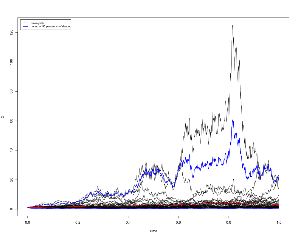
## Example 1: Ito sde
## dX(t) = 2*(3-X(t)) dt + 2*X(t) dW(t)
set.seed(1234)
f <- expression(2*(3-x) )
g <- expression(2*x)
res <- snssde1d(drift=f,diffusion=g,M=50,x0=1,N=1000)
res
## Sim <- res$X
summary(res)
plot(res,plot.type="single")
lines(time(res),mean(res),col=2,lwd=2)
lines(time(res),bconfint(res,level=0.95)[,1],col=4,lwd=2)
lines(time(res),bconfint(res,level=0.95)[,2],col=4,lwd=2)
legend("topleft",c("mean path",paste("bound of", 95,"percent confidence")),
inset = .01,col=c(2,4),lwd=2,cex=0.8)
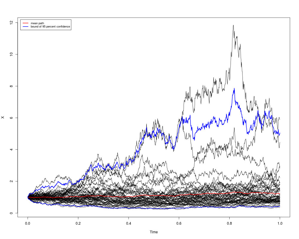
## Example 2: Stratonovich sde
## dX(t) = ((2-X(t))/(2-t)) dt + X(t) o dW(t)
set.seed(1234)
f <- expression((2-x)/(2-t))
g <- expression(x)
res1 <- snssde1d(type="str",drift=f,diffusion=g,M=50,x0=1,N=1000,
method="milstein")
res1
summary(res1)
plot(res1,plot.type="single")
lines(time(res1),mean(res1),col=2,lwd=2)
lines(time(res1),bconfint(res1,level=0.95)[,1],col=4,lwd=2)
lines(time(res1),bconfint(res1,level=0.95)[,2],col=4,lwd=2)
legend("topleft",c("mean path",paste("bound of", 95,"percent confidence")),
inset = .01,col=c(2,4),lwd=2,cex=0.8)
Results
R version 3.3.1 (2016-06-21) -- "Bug in Your Hair"
Copyright (C) 2016 The R Foundation for Statistical Computing
Platform: x86_64-pc-linux-gnu (64-bit)

R is free software and comes with ABSOLUTELY NO WARRANTY.
You are welcome to redistribute it under certain conditions.
Type 'license()' or 'licence()' for distribution details.

R is a collaborative project with many contributors.
Type 'contributors()' for more information and
'citation()' on how to cite R or R packages in publications.

Type 'demo()' for some demos, 'help()' for on-line help, or
'help.start()' for an HTML browser interface to help.
Type 'q()' to quit R.

> library(Sim.DiffProc)
Package 'Sim.DiffProc' version 3.2 loaded.
help(Sim.DiffProc) for summary information.
> png(filename="/home/ddbj/snapshot/RGM3/R_CC/result/Sim.DiffProc/snssde1d.Rd_%03d_medium.png", width=480, height=480)
> ### Name: snssde1d
> ### Title: Simulation of 1-Dim Stochastic Differential Equation
> ### Aliases: snssde1d snssde1d.default summary.snssde1d print.snssde1d
> ###   time.snssde1d mean.snssde1d median.snssde1d quantile.snssde1d
> ###   kurtosis.snssde1d skewness.snssde1d moment.snssde1d bconfint.snssde1d
> ###   plot.snssde1d points.snssde1d lines.snssde1d
> ### Keywords: sde ts mts
>
> ### ** Examples
>
>
> ## Example 1: Ito sde
> ## dX(t) = 2*(3-X(t)) dt + 2*X(t) dW(t)
> set.seed(1234)
>
> f <- expression(2*(3-x) )
> g <- expression(2*x)
> res <- snssde1d(drift=f,diffusion=g,M=50,x0=1,N=1000)
> res
Ito Sde 1D:
	| dX(t) = 2 * (3 - X(t)) * dt + 2 * X(t) * dW(t)
Method:
	| Euler scheme of order 0.5
Summary:
	| Size of process	| N  = 1000.
	| Number of simulation	| M  = 50.
	| Initial value		| x0 = 1.
	| Time of process	| t in [0,1].
	| Discretization	| Dt = 0.001.
> ## Sim <- res$X
> summary(res)

	Monte-Carlo Statistics for X(t) at final time T = 1

                                X
Mean                     3.142025
Variance                18.561062
Median                   1.715538
First quartile           1.083597
Third quartile           2.815213
Skewness                 2.992461
Kurtosis                11.728186
Moment of order 2       18.189840
Moment of order 3      239.294490
Moment of order 4     4040.512782
Moment of order 5    69072.177096
Bound conf Inf (95%)     0.654362
Bound conf Sup (95%)    17.057492
> plot(res,plot.type="single")
> lines(time(res),mean(res),col=2,lwd=2)
> lines(time(res),bconfint(res,level=0.95)[,1],col=4,lwd=2)
> lines(time(res),bconfint(res,level=0.95)[,2],col=4,lwd=2)
> legend("topleft",c("mean path",paste("bound of", 95,"percent confidence")),
+        inset = .01,col=c(2,4),lwd=2,cex=0.8)
>
> ## Example 2: Stratonovich sde
> ## dX(t) = ((2-X(t))/(2-t)) dt + X(t) o dW(t)
> set.seed(1234)
>
> f <- expression((2-x)/(2-t))
> g <- expression(x)
> res1 <- snssde1d(type="str",drift=f,diffusion=g,M=50,x0=1,N=1000,
+                  method="milstein")
> res1
Stratonovich Sde 1D:
	| dX(t) = (2 - X(t))/(2 - t) * dt + X(t) o dW(t)
Method:
	| Milstein scheme of order 1
Summary:
	| Size of process	| N  = 1000.
	| Number of simulation	| M  = 50.
	| Initial value		| x0 = 1.
	| Time of process	| t in [0,1].
	| Discretization	| Dt = 0.001.
> summary(res1)

	Monte-Carlo Statistics for X(t) at final time T = 1

                             X
Mean                  1.226419
Variance              0.995357
Median                0.875143
First quartile        0.734474
Third quartile        1.385116
Skewness              2.876349
Kurtosis             12.297469
Moment of order 2     0.975450
Moment of order 3     2.856342
Moment of order 4    12.183552
Moment of order 5    52.537073
Bound conf Inf (95%)  0.477809
Bound conf Sup (95%)  4.115370
> plot(res1,plot.type="single")
> lines(time(res1),mean(res1),col=2,lwd=2)
> lines(time(res1),bconfint(res1,level=0.95)[,1],col=4,lwd=2)
> lines(time(res1),bconfint(res1,level=0.95)[,2],col=4,lwd=2)
> legend("topleft",c("mean path",paste("bound of", 95,"percent confidence")),
+        inset = .01,col=c(2,4),lwd=2,cex=0.8)
>
>
>
>
>
> dev.off()
null device
          1
>
|