R Graphical Manual

Browse All

Last data update: 2014.03.03

R: Simulation of 2-Dim Stochastic Differential Equation

snssde2d

R Documentation

Simulation of 2-Dim Stochastic Differential Equation

Description

The (S3) generic function snssde2d of simulation of solutions to 2-dim stochastic differential equations of Ito or Stratonovich type, with different methods.

Usage

snssde2d(N, ...)
## Default S3 method:
snssde2d(N = 1000, M = 1, x0 = 0, y0 = 0, t0 = 0, T = 1, Dt, 
   driftx, diffx, drifty, diffy, alpha = 0.5, mu = 0.5, 
   type = c("ito", "str"), method = c("euler", "milstein", 
   "predcorr", "smilstein", "taylor", "heun", "rk1", "rk2",
   "rk3"), ...)
						   
						   
## S3 method for class 'snssde2d'
summary(object, ...)
## S3 method for class 'snssde2d'
time(x, ...)
## S3 method for class 'snssde2d'
mean(x, ...)
## S3 method for class 'snssde2d'
median(x, ...)
## S3 method for class 'snssde2d'
quantile(x, ...)
## S3 method for class 'snssde2d'
kurtosis(x, ...)
## S3 method for class 'snssde2d'
skewness(x, ...)
## S3 method for class 'snssde2d'
moment(x, order = 2, ...)
## S3 method for class 'snssde2d'
bconfint(x, level=0.95, ...)
## S3 method for class 'snssde2d'
plot(x, ...)
## S3 method for class 'snssde2d'
lines(x, ...)
## S3 method for class 'snssde2d'
points(x, ...)
## S3 method for class 'snssde2d'
plot2d(x, ...)
## S3 method for class 'snssde2d'
lines2d(x, ...)
## S3 method for class 'snssde2d'
points2d(x, ...)

Arguments

`N`	number of simulation steps.
`M`	number of trajectories.
`x0, y0`	initial value of the process X(t) and Y(t) at time `t0`.
`t0`	initial time.
`T`	final time.
`Dt`	time step of the simulation (discretization). If it is `missing` a default Dt = (T-t0)/N.
`driftx, drifty`	drift coefficient: an `expression` of three variables `t`, `x` and `y` for process X(t) and Y(t).
`diffx, diffy`	diffusion coefficient: an `expression` of three variables `t`, `x` and `y` for process X(t) and Y(t).
`alpha, mu`	weight of the predictor-corrector scheme; the default `alpha = 0.5` and `mu = 0.5`.
`type`	if `type="ito"` simulation sde of Ito type, else `type="str"` simulation sde of Stratonovich type; the default `type="ito"`.
`method`	numerical methods of simulation, the default `method = "euler"`.
`x, object`	an object inheriting from class `"snssde2d"`.
`order`	order of moment.
`level`	the confidence level required.
`...`	further arguments for (non-default) methods.

Details

The function snssde2d returns a mts x of length N+1; i.e. solution of the 2-dim sde (X(t),Y(t)) of Ito or Stratonovich types; If Dt is not specified, then the best discretization Dt = (T-t0)/N.

The 2-dim Ito stochastic differential equation is:

dX(t) = a(t,X(t),Y(t))*dt + b(t,X(t),Y(t))*dW1(t)

dY(t) = a(t,X(t),Y(t))*dt + b(t,X(t),Y(t))*dW2(t)

2-dim Stratonovich sde :

dX(t) = a(t,X(t),Y(t))*dt + b(t,X(t),Y(t)) o dW1(t)

dY(t) = a(t,X(t),Y(t))*dt + b(t,X(t),Y(t)) o dW2(t)

W1(t) and W2(t) two standard Brownian motion independent.

The methods of approximation are classified according to their different properties. Mainly two criteria of optimality are used in the literature: the strong and the weak (orders of) convergence. The method of simulation can be one among: Euler-Maruyama Order 0.5, Milstein Order 1, Milstein Second-Order, Predictor-Corrector method, Ito-Taylor Order 1.5, Heun Order 2 and Runge-Kutta Order 1, 2 and 3.

For more details see vignette("SDEs").

Value

snssde2d returns an object inheriting from class "snssde2d".

`X, Y`	an invisible `mts` (2-dim) object (X(t),Y(t)).
`driftx, drifty`	drift coefficient of X(t) and Y(t).
`diffx, diffy`	diffusion coefficient of X(t) and Y(t).
`type`	type of sde.
`method`	the numerical method used.

Author(s)

A.C. Guidoum, K. Boukhetala.

References

Friedman, A. (1975). Stochastic differential equations and applications. Volume 1, ACADEMIC PRESS.

Henderson, D. and Plaschko,P. (2006). Stochastic differential equations in science and engineering. World Scientific.

Allen, E. (2007). Modeling with Ito stochastic differential equations. Springer-Verlag.

Jedrzejewski, F. (2009). Modeles aleatoires et physique probabiliste. Springer-Verlag.

Iacus, S.M. (2008). Simulation and inference for stochastic differential equations: with R examples. Springer-Verlag, New York.

Kloeden, P.E, and Platen, E. (1989). A survey of numerical methods for stochastic differential equations. Stochastic Hydrology and Hydraulics, 3, 155–178.

Kloeden, P.E, and Platen, E. (1991a). Relations between multiple ito and stratonovich integrals. Stochastic Analysis and Applications, 9(3), 311–321.

Kloeden, P.E, and Platen, E. (1991b). Stratonovich and ito stochastic taylor expansions. Mathematische Nachrichten, 151, 33–50.

Kloeden, P.E, and Platen, E. (1995). Numerical Solution of Stochastic Differential Equations. Springer-Verlag, New York.

Oksendal, B. (2000). Stochastic Differential Equations: An Introduction with Applications. 5th edn. Springer-Verlag, Berlin.

Platen, E. (1980). Weak convergence of approximations of ito integral equations. Z Angew Math Mech. 60, 609–614.

Platen, E. and Bruti-Liberati, N. (2010). Numerical Solution of Stochastic Differential Equations with Jumps in Finance. Springer-Verlag, New York

Saito, Y, and Mitsui, T. (1993). Simulation of Stochastic Differential Equations. The Annals of the Institute of Statistical Mathematics, 3, 419–432.

Examples


## Example 1: Ito sde
## dX(t) = 4*(-1-X(t))*Y(t) dt + 0.2 dW1(t)
## dY(t) = 4*(1-Y(t))*X(t) dt + 0.2 dW2(t)
set.seed(1234)

fx <- expression(4*(-1-x)*y)
gx <- expression(0.2)
fy <- expression(4*(1-y)*x)
gy <- expression(0.2)

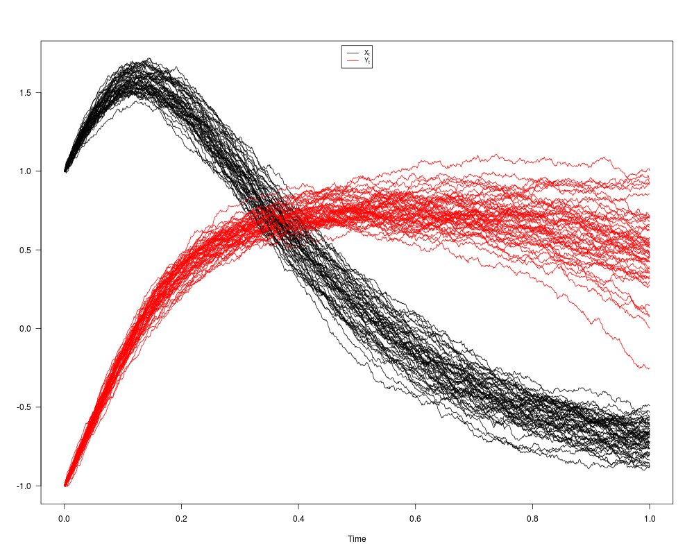
res <- snssde2d(driftx=fx,diffx=gx,drifty=fy,diffy=gy,x0=1,y0=-1,M=50)
res
summary(res)
plot(res)
dev.new()
plot2d(res) ## in plane (O,X,Y)

## Example 2: Stratonovich sde
## dX(t) = Y(t) dt + 0 o dW1(t)
## dY(t) = (4*(1-X(t)^2)*Y(t) - X(t) ) dt + 0.2 o dW2(t)
set.seed(1234)

fx <- expression( y )
gx <- expression( 0 )
fy <- expression( (4*( 1-x^2 )* y - x) )
gy <- expression( 0.2)

res1 <- snssde2d(driftx=fx,diffx=gx,drifty=fy,diffy=gy,type="str",T=100,
                 ,N=10000)
res1
plot(res1,pos=2)
dev.new()
plot(res1,union = FALSE)
dev.new()
plot2d(res1,type="n") ## in plane (O,X,Y)
points2d(res1,col=rgb(0,100,0,50,maxColorValue=255), pch=16)

Results


R version 3.3.1 (2016-06-21) -- "Bug in Your Hair"
Copyright (C) 2016 The R Foundation for Statistical Computing
Platform: x86_64-pc-linux-gnu (64-bit)

R is free software and comes with ABSOLUTELY NO WARRANTY.
You are welcome to redistribute it under certain conditions.
Type 'license()' or 'licence()' for distribution details.

R is a collaborative project with many contributors.
Type 'contributors()' for more information and
'citation()' on how to cite R or R packages in publications.

Type 'demo()' for some demos, 'help()' for on-line help, or
'help.start()' for an HTML browser interface to help.
Type 'q()' to quit R.

> library(Sim.DiffProc)
Package 'Sim.DiffProc' version 3.2 loaded.
help(Sim.DiffProc) for summary information.
> png(filename="/home/ddbj/snapshot/RGM3/R_CC/result/Sim.DiffProc/snssde2d.Rd_%03d_medium.png", width=480, height=480)
> ### Name: snssde2d
> ### Title: Simulation of 2-Dim Stochastic Differential Equation
> ### Aliases: snssde2d snssde2d.default summary.snssde2d print.snssde2d
> ###   time.snssde2d mean.snssde2d median.snssde2d quantile.snssde2d
> ###   kurtosis.snssde2d skewness.snssde2d moment.snssde2d bconfint.snssde2d
> ###   plot.snssde2d points.snssde2d lines.snssde2d plot2d.snssde2d
> ###   points2d.snssde2d lines2d.snssde2d
> ### Keywords: sde ts mts
> 
> ### ** Examples
> 
> 
> ## Example 1: Ito sde
> ## dX(t) = 4*(-1-X(t))*Y(t) dt + 0.2 dW1(t)
> ## dY(t) = 4*(1-Y(t))*X(t) dt + 0.2 dW2(t)
> set.seed(1234)
> 
> fx <- expression(4*(-1-x)*y)
> gx <- expression(0.2)
> fy <- expression(4*(1-y)*x)
> gy <- expression(0.2)
> 
> res <- snssde2d(driftx=fx,diffx=gx,drifty=fy,diffy=gy,x0=1,y0=-1,M=50)
> res
Ito Sde 2D:
	| dX(t) = 4 * (-1 - X(t)) * Y(t) * dt + 0.2 * dW1(t)
	| dY(t) = 4 * (1 - Y(t)) * X(t) * dt + 0.2 * dW2(t)
Method:
	| Euler scheme of order 0.5
Summary:
	| Size of process	| N  = 1000.
	| Number of simulation	| M  = 50.
	| Initial values	| (x0,y0) = (1,-1).
	| Time of process	| t in [0,1].
	| Discretization	| Dt = 0.001.
> summary(res)

	Monte-Carlo Statistics for (X(t),Y(t)) at final time T = 1

                             X         Y
Mean                 -0.694103  0.499599
Variance              0.009456  0.061898
Median               -0.676093  0.482477
First quartile       -0.762466  0.364142
Third quartile       -0.619803  0.639682
Skewness             -0.209476 -0.302930
Kurtosis              2.215742  3.655694
Moment of order 2     0.009267  0.060660
Moment of order 3    -0.000193 -0.004665
Moment of order 4     0.000198  0.014006
Moment of order 5    -0.000007 -0.004024
Bound conf Inf (95%) -0.874868  0.017159
Bound conf Sup (95%) -0.538741  0.945916
> plot(res)
> dev.new()
Error in dev.new() : no suitable unused file name for pdf()
Execution halted