R Graphical Manual

Browse All

Last data update: 2014.03.03

R: Stochastic Integrals

st.int

R Documentation

Stochastic Integrals

Description

The (S3) generic function st.int of simulation of stochastic integrals of Ito or Stratonovich type.

Usage

st.int(expr, ...)
## Default S3 method:
st.int(expr, lower = 0, upper = 1, M = 1, subdivisions = 1000L, 
               type = c("ito", "str"), ...)

## S3 method for class 'st.int'
summary(object, ...)
## S3 method for class 'st.int'
time(x, ...)
## S3 method for class 'st.int'
mean(x, ...)
## S3 method for class 'st.int'
median(x, ...)
## S3 method for class 'st.int'
quantile(x, ...)
## S3 method for class 'st.int'
kurtosis(x, ...)
## S3 method for class 'st.int'
skewness(x, ...)
## S3 method for class 'st.int'
moment(x, order = 2, ...)
## S3 method for class 'st.int'
bconfint(x, level=0.95, ...)
## S3 method for class 'st.int'
plot(x, ...)
## S3 method for class 'st.int'
lines(x, ...)
## S3 method for class 'st.int'
points(x, ...)

Arguments

`expr`	an `expression` of two variables `t` (time) and `w` (`w`: standard Brownian motion).
`lower, upper`	the lower and upper end points of the interval to be integrate.
`M`	number of trajectories.
`subdivisions`	the maximum number of subintervals.
`type`	Ito or Stratonovich integration.
`x, object`	an object inheriting from class `"st.int"`.
`order`	order of moment.
`level`	the confidence level required.
`...`	further arguments for (non-default) methods.

Details

The function st.int returns a ts x of length N+1; i.e. simulation of stochastic integrals of Ito or Stratonovich type.

The Ito interpretation is:

int(f(s)*dw(s),t0,T) = sum(f(t(i-1)) * (W(t(i)) - W(t(i-1))),i=1,…,N)

The Stratonovich interpretation is:

int(f(s) o dw(s),t0,T) = sum(f((t(i)+t(i-1))/2) * (W(t(i)) - W(t(i-1))),i=1,…,N)

For more details see vignette("SDEs").

Value

st.int returns an object inheriting from class "st.int".

`X`	the final simulation of the integral, an invisible `ts` object.
`fun`	function to be integrated.
`type`	type of stochastic integral.
`subdivisions`	the number of subintervals produced in the subdivision process.

Author(s)

A.C. Guidoum, K. Boukhetala.

References

Ito, K. (1944). Stochastic integral. Proc. Jap. Acad, Tokyo, 20, 19–529.

Kloeden, P.E, and Platen, E. (1995). Numerical Solution of Stochastic Differential Equations. Springer-Verlag, New York.

Oksendal, B. (2000). Stochastic Differential Equations: An Introduction with Applications. 5th edn. Springer-Verlag, Berlin.

Examples


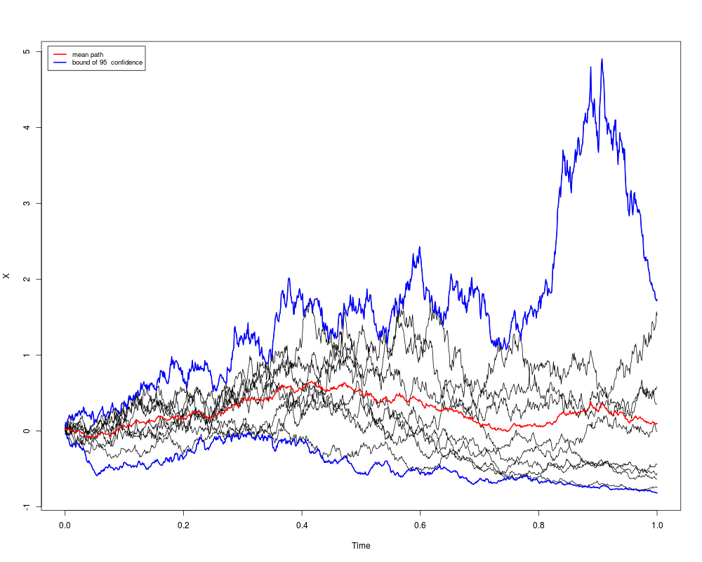
## Example 1: Ito integral
## f(t,w(t)) = int(exp(w(t) - 0.5*t) * dw(s)) with t in [0,1]
set.seed(1234)

fexpr <- expression( exp(w-0.5*t) )
res <- st.int(fexpr,type="ito",M=10,lower=0,upper=1)
res
## res$X 
summary(res)
## Display
plot(res,plot.type="single")
lines(time(res),mean(res),col=2,lwd=2)
lines(time(res),bconfint(res,level=0.95)[,1],col=4,lwd=2)
lines(time(res),bconfint(res,level=0.95)[,2],col=4,lwd=2)
legend("topleft",c("mean path",paste("bound of", 95," confidence")),
        inset = .01,col=c(2,4),lwd=2,cex=0.8)

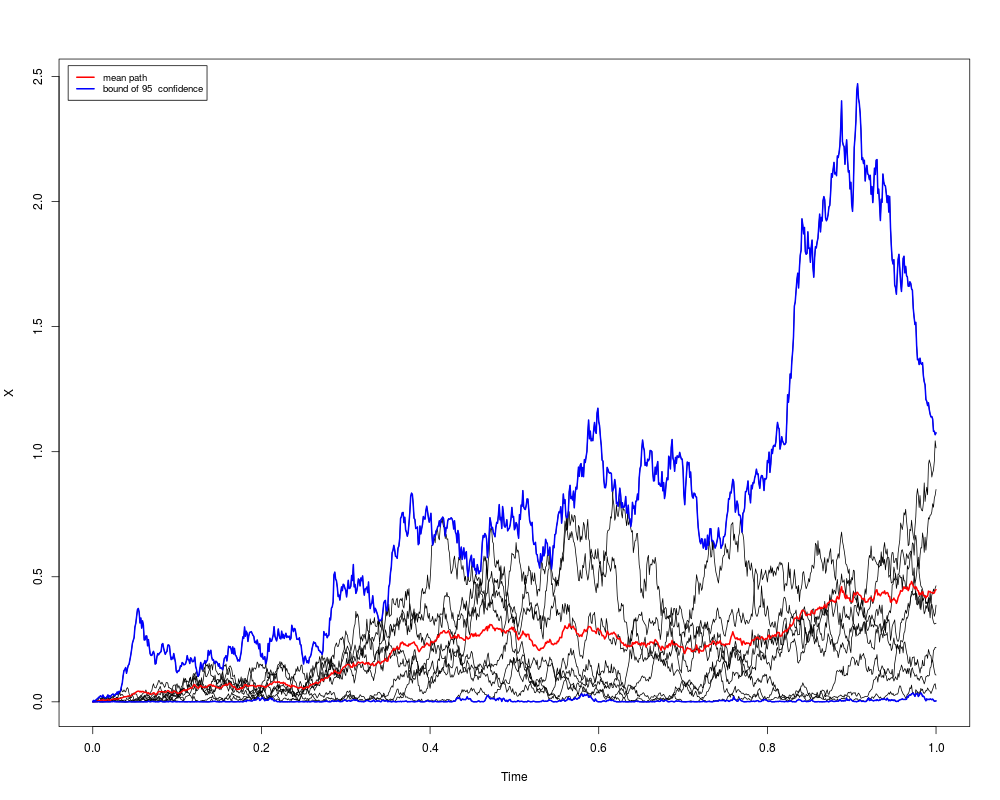
## Example 2: Stratonovich integral
## f(t,w(t)) = int(w(s)  o dw(s)) with t in [0,1]
set.seed(1234)

fexpr <- expression( w )
res1 <- st.int(fexpr,type="str",M=10,lower=0,upper=1)
res1
## res1$X 
summary(res1)
## Display
plot(res1,plot.type="single")
lines(time(res1),mean(res1),col=2,lwd=2)
lines(time(res1),bconfint(res1,level=0.95)[,1],col=4,lwd=2)
lines(time(res1),bconfint(res1,level=0.95)[,2],col=4,lwd=2)
legend("topleft",c("mean path",paste("bound of", 95," confidence")),
       inset = .01,col=c(2,4),lwd=2,cex=0.8)

Results


R version 3.3.1 (2016-06-21) -- "Bug in Your Hair"
Copyright (C) 2016 The R Foundation for Statistical Computing
Platform: x86_64-pc-linux-gnu (64-bit)

R is free software and comes with ABSOLUTELY NO WARRANTY.
You are welcome to redistribute it under certain conditions.
Type 'license()' or 'licence()' for distribution details.

R is a collaborative project with many contributors.
Type 'contributors()' for more information and
'citation()' on how to cite R or R packages in publications.

Type 'demo()' for some demos, 'help()' for on-line help, or
'help.start()' for an HTML browser interface to help.
Type 'q()' to quit R.

> library(Sim.DiffProc)
Package 'Sim.DiffProc' version 3.2 loaded.
help(Sim.DiffProc) for summary information.
> png(filename="/home/ddbj/snapshot/RGM3/R_CC/result/Sim.DiffProc/st.int.Rd_%03d_medium.png", width=480, height=480)
> ### Name: st.int
> ### Title: Stochastic Integrals
> ### Aliases: st.int st.int.default summary.st.int print.st.int time.st.int
> ###   mean.st.int median.st.int quantile.st.int kurtosis.st.int
> ###   skewness.st.int moment.st.int bconfint.st.int plot.st.int
> ###   points.st.int lines.st.int
> ### Keywords: sde ts
> 
> ### ** Examples
> 
> 
> ## Example 1: Ito integral
> ## f(t,w(t)) = int(exp(w(t) - 0.5*t) * dw(s)) with t in [0,1]
> set.seed(1234)
> 
> fexpr <- expression( exp(w-0.5*t) )
> res <- st.int(fexpr,type="ito",M=10,lower=0,upper=1)
> res
Ito integral:
	| X(t)   = integral (f(s,w) * dw(s))
	| f(t,w) = exp(w - 0.5 * t)
Summary:
	| Number of subintervals	 = 1000.
	| Number of simulations		 = 10.
	| Limits of integration		 = [0,1].
	| Discretization		 = 0.001.
> ## res$X 
> summary(res)

	Monte-Carlo Statistics for X(t) at final time T = 1

| Process mean			 = 0.09727184
| Process variance		 = 0.8688662
| Process median		 = -0.2274052
| Process first quartile	 = -0.615378
| Process third quartile	 = 0.5267111
| Process skewness		 = 0.6357756
| Process kurtosis		 = 1.726596
| Process moment of order 2	 = 0.7819796
| Process moment of order 3	 = 0.5149123
| Process moment of order 4	 = 1.303456
| Process moment of order 5	 = 1.5976
| Bound of confidence (95%)	 = [-0.8042869,1.682069]
  for the trajectories
> ## Display
> plot(res,plot.type="single")
> lines(time(res),mean(res),col=2,lwd=2)
> lines(time(res),bconfint(res,level=0.95)[,1],col=4,lwd=2)
> lines(time(res),bconfint(res,level=0.95)[,2],col=4,lwd=2)
> legend("topleft",c("mean path",paste("bound of", 95," confidence")),
+         inset = .01,col=c(2,4),lwd=2,cex=0.8)
> 
> ## Example 2: Stratonovich integral
> ## f(t,w(t)) = int(w(s)  o dw(s)) with t in [0,1]
> set.seed(1234)
> 
> fexpr <- expression( w )
> res1 <- st.int(fexpr,type="str",M=10,lower=0,upper=1)
> res1
Stratonovich integral:
	| X(t)   = integral (f(s,w) o dw(s))
	| f(t,w) = w
Summary:
	| Number of subintervals	 = 1000.
	| Number of simulations		 = 10.
	| Limits of integration		 = [0,1].
	| Discretization		 = 0.001.
> ## res1$X 
> summary(res1)

	Monte-Carlo Statistics for X(t) at final time T = 1

| Process mean			 = 0.4482631
| Process variance		 = 0.1581149
| Process median		 = 0.3504116
| Process first quartile	 = 0.1344491
| Process third quartile	 = 0.7527277
| Process skewness		 = 0.4580159
| Process kurtosis		 = 1.458378
| Process moment of order 2	 = 0.1423034
| Process moment of order 3	 = 0.02879651
| Process moment of order 4	 = 0.03645993
| Process moment of order 5	 = 0.01333736
| Bound of confidence (95%)	 = [0.01432213,1.061882]
  for the trajectories
> ## Display
> plot(res1,plot.type="single")
> lines(time(res1),mean(res1),col=2,lwd=2)
> lines(time(res1),bconfint(res1,level=0.95)[,1],col=4,lwd=2)
> lines(time(res1),bconfint(res1,level=0.95)[,2],col=4,lwd=2)
> legend("topleft",c("mean path",paste("bound of", 95," confidence")),
+        inset = .01,col=c(2,4),lwd=2,cex=0.8)
> 
> 
> 
> 
> 
> dev.off()
null device 
          1 
>