Multivariate Normal Random Numbers with Exact Parameters

Description

Random numbers of the multivariate normal distribution with EXACT mean vector, EXACT variance vector and approximate correlation matrix. This function is based on the function rmvnorm of the package mvtnorm.

Usage

ermvnorm(n, mean, sd, corr = diag(rep(1, length(mean))), mnt = 10000)

Arguments

Details

Unfortunately, it's very common to present only summary statistics in the literature when evaluating real data. This makes it hard to retrace or to verify the related statistical evaluation. Also, the use of such data as an example for other statistical tests is hardly possible. For that reason, ermvnorm allows to reproduce data by simulation. In contrast to rmvnorm of the package mvtnorm, the function ermvnorm produces random numbers which have EXACTLY the same paramer values as specified by mean and sd. The correlation matrix corr is met only approximately.

The simple idea behind ermvnorm is to apply rmvnorm of the package mvtnorm, but only for the first n-2 random numbers. The remaining 2 numbers are obtained by solving a quadratic equation to achieve the specified values for the mean vector and for the vector of standard deviations. Depending on the n-2 random numbers, the underlying quadratic equation can possibly have no solution. In this case, ermvnorm creates a new set of n-2 random numbers until a valid data set is obtained, or until the maximum number of tries mnt is reached.

Value

A matrix of random numbers with dimension n * length(mean).

Note

This function is to be used only with caution. Normally, random numbers with exact mean and standard deviation are not intended to be used. For example, simulations concerning type I error or power of statistical tests cannot be based on ermvnorm.

Author(s)

Gemechis Djira Dilba and Mario Hasler

References

Hothorn, T. et al. (2001): On Multivariate t and Gauss Probabilities in R. R News 1, 27–29.

See Also

rmvnorm, rcm

Examples

# Example 1:
# A dataset representing one endpoint.

set.seed(1234)
dataset1 <- ermvnorm(n=10,mean=100,sd=10)
dataset1
mean(dataset1)
sd(dataset1)

# Example 2:
# A dataset representing two correlated endpoints.

set.seed(5678)
dataset2 <- ermvnorm(n=10,mean=c(10,120),sd=c(1,10),corr=rbind(c(1,0.7),c(0.7,1)))
dataset2
mean(dataset2[,1]); mean(dataset2[,2])
sd(dataset2[,1]); sd(dataset2[,2])
round(cor(dataset2),3)
pairs(dataset2)

# Example 3:
# A dataset representing three uncorrelated endpoints.

set.seed(9101)
dataset3 <- ermvnorm(n=20,mean=c(1,12,150),sd=c(0.5,2,20))
dataset3
mean(dataset3[,1]); mean(dataset3[,2]); mean(dataset3[,3])
sd(dataset3[,1]); sd(dataset3[,2]); sd(dataset3[,3])
pairs(dataset3)

# Example 4:
# A dataset representing four randomly correlated endpoints.

set.seed(1121)
dataset4 <- ermvnorm(n=10,mean=c(2,10,50,120),sd=c(1,4,8,10),corr=rcm(ncol=4))
dataset4
mean(dataset4[,1]); mean(dataset4[,2]); mean(dataset4[,3]); mean(dataset4[,4])
sd(dataset4[,1]); sd(dataset4[,2]); sd(dataset4[,3]); sd(dataset4[,4])
round(cor(dataset4),3)
pairs(dataset4)

Results

R version 3.3.1 (2016-06-21) -- "Bug in Your Hair"
Copyright (C) 2016 The R Foundation for Statistical Computing
Platform: x86_64-pc-linux-gnu (64-bit)

R is free software and comes with ABSOLUTELY NO WARRANTY.
You are welcome to redistribute it under certain conditions.
Type 'license()' or 'licence()' for distribution details.

R is a collaborative project with many contributors.
Type 'contributors()' for more information and
'citation()' on how to cite R or R packages in publications.

Type 'demo()' for some demos, 'help()' for on-line help, or
'help.start()' for an HTML browser interface to help.
Type 'q()' to quit R.

> library(SimComp)
> png(filename="/home/ddbj/snapshot/RGM3/R_CC/result/SimComp/ermvnorm.Rd_%03d_medium.png", width=480, height=480)
> ### Name: ermvnorm
> ### Title: Multivariate Normal Random Numbers with Exact Parameters
> ### Aliases: ermvnorm
> ### Keywords: datagen distribution
> 
> ### ** Examples
> 
> # Example 1:
> # A dataset representing one endpoint.
> 
> set.seed(1234)
> dataset1 <- ermvnorm(n=10,mean=100,sd=10)
> dataset1
           [,1]
 [1,]  94.35548
 [2,]  91.09962
 [3,]  95.22807
 [4,]  90.01614
 [5,]  92.23746
 [6,] 100.64459
 [7,] 109.59494
 [8,]  98.89715
 [9,] 106.13461
[10,] 121.79194
> mean(dataset1)
[1] 100
> sd(dataset1)
[1] 10
> 
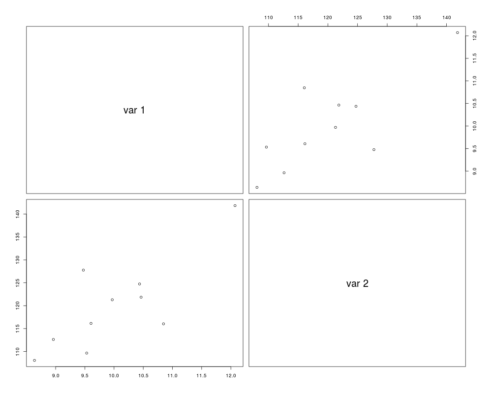
> # Example 2:
> # A dataset representing two correlated endpoints.
> 
> set.seed(5678)
> dataset2 <- ermvnorm(n=10,mean=c(10,120),sd=c(1,10),corr=rbind(c(1,0.7),c(0.7,1)))
> dataset2
           [,1]     [,2]
 [1,] 10.436945 124.7436
 [2,]  8.961315 112.6236
 [3,]  9.605753 116.1367
 [4,]  9.474919 127.7627
 [5,] 10.463401 121.8539
 [6,] 10.846991 116.0376
 [7,]  8.638005 108.0569
 [8,]  9.531624 109.6470
 [9,]  9.969430 121.2914
[10,] 12.071617 141.8466
> mean(dataset2[,1]); mean(dataset2[,2])
[1] 10
[1] 120
> sd(dataset2[,1]); sd(dataset2[,2])
[1] 1
[1] 10
> round(cor(dataset2),3)
      [,1]  [,2]
[1,] 1.000 0.789
[2,] 0.789 1.000
> pairs(dataset2)
> 
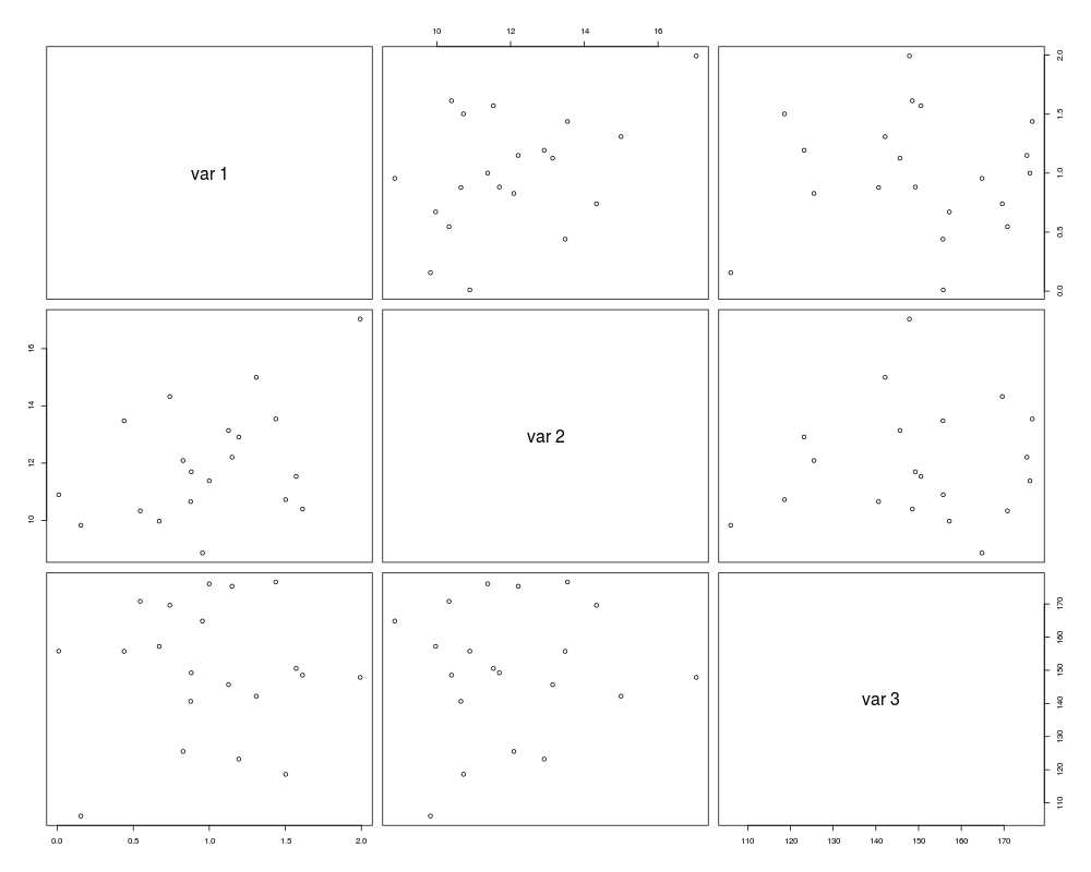
> # Example 3:
> # A dataset representing three uncorrelated endpoints.
> 
> set.seed(9101)
> dataset3 <- ermvnorm(n=20,mean=c(1,12,150),sd=c(0.5,2,20))
> dataset3
           [,1]      [,2]     [,3]
 [1,] 0.9998719 11.380115 176.0773
 [2,] 0.7403547 14.330042 169.5992
 [3,] 1.5709859 11.534055 150.5554
 [4,] 0.5460682 10.331224 170.8062
 [5,] 0.8276285 12.089328 125.5125
 [6,] 1.1938283 12.912070 123.2066
 [7,] 0.9552236  8.857654 164.8589
 [8,] 0.8773945 10.653175 140.6339
 [9,] 0.8817714 11.695834 149.2280
[10,] 0.0100066 10.894319 155.7632
[11,] 1.4374201 13.543762 176.6189
[12,] 1.5018459 10.722467 118.6061
[13,] 0.6711652  9.969019 157.2028
[14,] 1.1264022 13.141976 145.6454
[15,] 1.1497216 12.205792 175.3696
[16,] 1.3088858 14.997851 142.1800
[17,] 0.4400495 13.480476 155.7131
[18,] 1.6130400 10.396497 148.5401
[19,] 0.1558448  9.826444 106.0264
[20,] 1.9924913 17.037898 147.8563
> mean(dataset3[,1]); mean(dataset3[,2]); mean(dataset3[,3])
[1] 1
[1] 12
[1] 150
> sd(dataset3[,1]); sd(dataset3[,2]); sd(dataset3[,3])
[1] 0.5
[1] 2
[1] 20
> pairs(dataset3)
> 
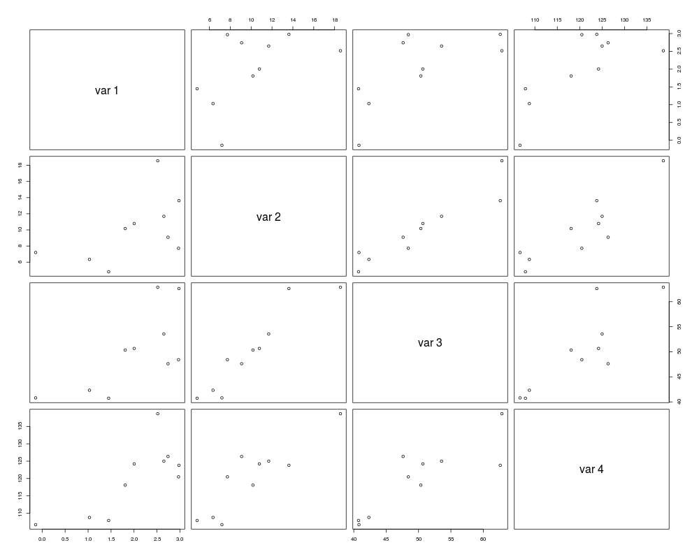
> # Example 4:
> # A dataset representing four randomly correlated endpoints.
> 
> set.seed(1121)
> dataset4 <- ermvnorm(n=10,mean=c(2,10,50,120),sd=c(1,4,8,10),corr=rcm(ncol=4))
> dataset4
            [,1]      [,2]     [,3]     [,4]
 [1,]  2.9683978  7.725205 48.42291 120.4834
 [2,]  2.6494078 11.684351 53.56060 125.0098
 [3,]  2.0036845 10.790225 50.66751 124.2170
 [4,]  2.9783659 13.620772 62.62520 123.8164
 [5,]  1.4475155  4.816900 40.73623 107.8946
 [6,]  2.7397549  9.088985 47.61865 126.3443
 [7,]  1.0302284  6.343625 42.33113 108.7764
 [8,]  1.8080773 10.170706 50.35773 118.0953
 [9,] -0.1417155  7.197329 40.79931 106.6884
[10,]  2.5162835 18.561902 62.88073 138.6744
> mean(dataset4[,1]); mean(dataset4[,2]); mean(dataset4[,3]); mean(dataset4[,4])
[1] 2
[1] 10
[1] 50
[1] 120
> sd(dataset4[,1]); sd(dataset4[,2]); sd(dataset4[,3]); sd(dataset4[,4])
[1] 1
[1] 4
[1] 8
[1] 10
> round(cor(dataset4),3)
      [,1]  [,2]  [,3]  [,4]
[1,] 1.000 0.516 0.697 0.758
[2,] 0.516 1.000 0.938 0.887
[3,] 0.697 0.938 1.000 0.852
[4,] 0.758 0.887 0.852 1.000
> pairs(dataset4)
> 
> 
> 
> 
> 
> dev.off()
null device 
          1 
>