Supported by Dr. Osamu Ogasawara and  . . |
|
Last data update: 2014.03.03 |
Plot function for SimCi-objectsDescriptionA plot of the results of Usage## S3 method for class 'SimCi' plot(x, xlim, xlab, ylim, ...) Arguments
ValueA plot of the confidence intervals of a "SimCi" object. Author(s)Christof Kluss and Mario Hasler See Also
Examples
# Example 1:
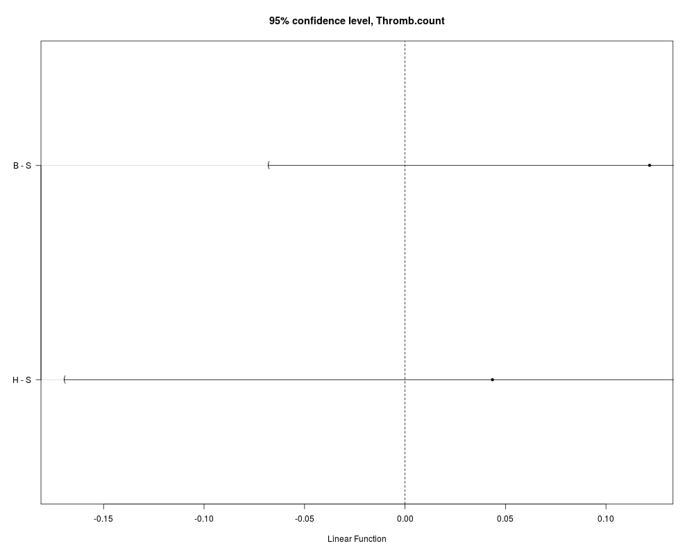
# Simultaneous confidence intervals related to a comparison of the groups
# B and H against the standard S, on endpoint Thromb.count, assuming unequal
# variances for the groups. This is an extension of the well-known Dunnett-
# intervals to the case of heteroscedasticity.
data(coagulation)
interv1 <- SimCiDiff(data=coagulation, grp="Group", resp="Thromb.count",
type="Dunnett", base=3, alternative="greater", covar.equal=FALSE)
interv1
plot(interv1)
# Example 2:
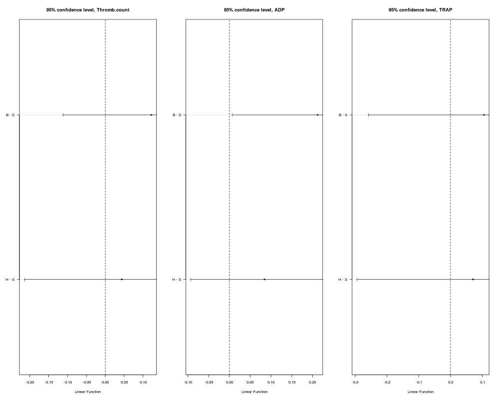
# Simultaneous confidence intervals related to a comparisons of the groups
# B and H against the standard S, simultaneously on all endpoints, assuming
# unequal covariance matrices for the groups. This is an extension of the well-
# known Dunnett-intervals to the case of heteroscedasticity and multiple
# endpoints.
data(coagulation)
interv2 <- SimCiDiff(data=coagulation, grp="Group", resp=c("Thromb.count","ADP","TRAP"),
type="Dunnett", base=3, alternative="greater", covar.equal=FALSE)
summary(interv2)
par(mfrow=c(1,3)); plot(interv2)
# Example 3:
# Simultaneous confidence intervals for ratios of means, related to an all-pair
# comparison of the groups B, H and S, simultaneously on all endpoints, assuming unequal
# covariance matrices for the groups. This is an extension of the well-known Tukey-
# intervals to the case of heteroscedasticity and multiple endpoints, and in terms of
# ratios of means instead of differences.
data(coagulation)
interv3 <- SimCiRat(data=coagulation, grp="Group", resp=c("Thromb.count","ADP","TRAP"),
type="Tukey", alternative="two.sided", covar.equal=FALSE)
summary(interv3)
par(mfrow=c(3,1)); plot(interv3)
Results
R version 3.3.1 (2016-06-21) -- "Bug in Your Hair"
Copyright (C) 2016 The R Foundation for Statistical Computing
Platform: x86_64-pc-linux-gnu (64-bit)

R is free software and comes with ABSOLUTELY NO WARRANTY.
You are welcome to redistribute it under certain conditions.
Type 'license()' or 'licence()' for distribution details.

R is a collaborative project with many contributors.
Type 'contributors()' for more information and
'citation()' on how to cite R or R packages in publications.

Type 'demo()' for some demos, 'help()' for on-line help, or
'help.start()' for an HTML browser interface to help.
Type 'q()' to quit R.

> library(SimComp)
> png(filename="/home/ddbj/snapshot/RGM3/R_CC/result/SimComp/plot.SimCi.Rd_%03d_medium.png", width=480, height=480)
> ### Name: plot.SimCi
> ### Title: Plot function for SimCi-objects
> ### Aliases: plot.SimCi
> ### Keywords: print
>
> ### ** Examples
>
> # Example 1:
> # Simultaneous confidence intervals related to a comparison of the groups
> # B and H against the standard S, on endpoint Thromb.count, assuming unequal
> # variances for the groups. This is an extension of the well-known Dunnett-
> # intervals to the case of heteroscedasticity.
>
> data(coagulation)
>
> interv1 <- SimCiDiff(data=coagulation, grp="Group", resp="Thromb.count",
+   type="Dunnett", base=3, alternative="greater", covar.equal=FALSE)
> interv1

Simultaneous 95% confidence intervals for differences of means of multiple endpoints
Assumption: Heterogeneous covariance matrices for the groups

  comparison     endpoint estimate lower.raw upper.raw   lower upper
1      B - S Thromb.count   0.1217   -0.0367       Inf -0.0681   Inf
2      H - S Thromb.count   0.0435   -0.1344       Inf -0.1695   Inf

> plot(interv1)
>
> # Example 2:
> # Simultaneous confidence intervals related to a comparisons of the groups
> # B and H against the standard S, simultaneously on all endpoints, assuming
> # unequal covariance matrices for the groups. This is an extension of the well-
> # known Dunnett-intervals to the case of heteroscedasticity and multiple
> # endpoints.
>
> data(coagulation)
>
> interv2 <- SimCiDiff(data=coagulation, grp="Group", resp=c("Thromb.count","ADP","TRAP"),
+   type="Dunnett", base=3, alternative="greater", covar.equal=FALSE)
> summary(interv2)

Contrast matrix:

	 Multiple Comparisons of Means: Dunnett Contrasts

      B H  S
B - S 1 0 -1
H - S 0 1 -1

Estimated covariance matrices of the data:
$B
             Thromb.count    ADP    TRAP
Thromb.count       0.0626 0.0565 -0.0102
ADP                0.0565 0.0638  0.0054
TRAP              -0.0102 0.0054  0.0963

$H
             Thromb.count    ADP   TRAP
Thromb.count       0.0943 0.0637 0.0663
ADP                0.0637 0.0518 0.0446
TRAP               0.0663 0.0446 0.1157

$S
             Thromb.count    ADP   TRAP
Thromb.count       0.0318 0.0132 0.0598
ADP                0.0132 0.0079 0.0269
TRAP               0.0598 0.0269 0.1376


Estimated correlation matrices of the data:
$B
             Thromb.count    ADP    TRAP
Thromb.count       1.0000 0.8937 -0.1314
ADP                0.8937 1.0000  0.0687
TRAP              -0.1314 0.0687  1.0000

$H
             Thromb.count    ADP   TRAP
Thromb.count       1.0000 0.9121 0.6348
ADP                0.9121 1.0000 0.5770
TRAP               0.6348 0.5770 1.0000

$S
             Thromb.count    ADP   TRAP
Thromb.count       1.0000 0.8338 0.9033
ADP                0.8338 1.0000 0.8161
TRAP               0.9033 0.8161 1.0000


Estimated correlation matrix of the comparisons:
       [,1]   [,2]   [,3]   [,4]   [,5]   [,6]
[1,] 1.0000 0.8494 0.3122 0.2833 0.1708 0.3755
[2,] 0.8494 1.0000 0.2387 0.1335 0.1158 0.1917
[3,] 0.3122 0.2387 1.0000 0.3417 0.2232 0.5550
[4,] 0.2833 0.1335 0.3417 1.0000 0.8869 0.7054
[5,] 0.1708 0.1158 0.2232 0.8869 1.0000 0.5818
[6,] 0.3755 0.1917 0.5550 0.7054 0.5818 1.0000

  comparison     endpoint estimate lower.raw upper.raw   lower upper
1      B - S Thromb.count   0.1217   -0.0367       Inf -0.1119   Inf
2      B - S          ADP   0.2121    0.0691       Inf  0.0067   Inf
3      B - S         TRAP   0.1053   -0.1395       Inf -0.2582   Inf
4      H - S Thromb.count   0.0435   -0.1344       Inf -0.2139   Inf
5      H - S          ADP   0.0842   -0.0398       Inf -0.0928   Inf
6      H - S         TRAP   0.0711   -0.1784       Inf -0.2941   Inf

> par(mfrow=c(1,3)); plot(interv2)
>
> # Example 3:
> # Simultaneous confidence intervals for ratios of means, related to an all-pair
> # comparison of the groups B, H and S, simultaneously on all endpoints, assuming unequal
> # covariance matrices for the groups. This is an extension of the well-known Tukey-
> # intervals to the case of heteroscedasticity and multiple endpoints, and in terms of
> # ratios of means instead of differences.
>
> data(coagulation)
>
> interv3 <- SimCiRat(data=coagulation, grp="Group", resp=c("Thromb.count","ADP","TRAP"),
+   type="Tukey", alternative="two.sided", covar.equal=FALSE)
> summary(interv3)

Numerator contrast matrix:
    B H S
H/B 0 1 0
S/B 0 0 1
S/H 0 0 1

Denominator contrast matrix:
    B H S
H/B 1 0 0
S/B 1 0 0
S/H 0 1 0

Estimated covariance matrices of the data:
$B
             Thromb.count    ADP    TRAP
Thromb.count       0.0626 0.0565 -0.0102
ADP                0.0565 0.0638  0.0054
TRAP              -0.0102 0.0054  0.0963

$H
             Thromb.count    ADP   TRAP
Thromb.count       0.0943 0.0637 0.0663
ADP                0.0637 0.0518 0.0446
TRAP               0.0663 0.0446 0.1157

$S
             Thromb.count    ADP   TRAP
Thromb.count       0.0318 0.0132 0.0598
ADP                0.0132 0.0079 0.0269
TRAP               0.0598 0.0269 0.1376


Estimated correlation matrices of the data:
$B
             Thromb.count    ADP    TRAP
Thromb.count       1.0000 0.8937 -0.1314
ADP                0.8937 1.0000  0.0687
TRAP              -0.1314 0.0687  1.0000

$H
             Thromb.count    ADP   TRAP
Thromb.count       1.0000 0.9121 0.6348
ADP                0.9121 1.0000 0.5770
TRAP               0.6348 0.5770 1.0000

$S
             Thromb.count    ADP   TRAP
Thromb.count       1.0000 0.8338 0.9033
ADP                0.8338 1.0000 0.8161
TRAP               0.9033 0.8161 1.0000


Estimated correlation matrix of the comparisons:
         [,1]    [,2]    [,3]    [,4]   [,5]    [,6]    [,7]    [,8]    [,9]
 [1,]  1.0000  0.8966  0.3141  0.4869 0.5076 -0.0492 -0.6719 -0.6593 -0.3202
 [2,]  0.8966  1.0000  0.3320  0.5023 0.6555  0.0297 -0.5467 -0.6448 -0.2596
 [3,]  0.3141  0.3320  1.0000 -0.0699 0.0426  0.4093 -0.4001 -0.3912 -0.4731
 [4,]  0.4869  0.5023 -0.0699  1.0000 0.8494  0.3781  0.3198  0.2025  0.4258
 [5,]  0.5076  0.6555  0.0426  0.8494 1.0000  0.2918  0.1697  0.1545  0.2448
 [6,] -0.0492  0.0297  0.4093  0.3781 0.2918  1.0000  0.3740  0.2566  0.6102
 [7,] -0.6719 -0.5467 -0.4001  0.3198 0.1697  0.3740  1.0000  0.8869  0.7084
 [8,] -0.6593 -0.6448 -0.3912  0.2025 0.1545  0.2566  0.8869  1.0000  0.5874
 [9,] -0.3202 -0.2596 -0.4731  0.4258 0.2448  0.6102  0.7084  0.5874  1.0000

  comparison     endpoint estimate lower.raw upper.raw  lower upper
1        H/B Thromb.count   0.9213    0.7046    1.1853 0.6276 1.309
2        H/B          ADP   0.8746    0.7020    1.0905 0.6415 1.194
3        H/B         TRAP   0.9589    0.6675    1.3617 0.5682 1.580
4        S/B Thromb.count   0.8775    0.7201    1.0803 0.6577 1.197
5        S/B          ADP   0.7921    0.6714    0.9547 0.6294 1.042
6        S/B         TRAP   0.8733    0.5726    1.2760 0.4497 1.532
7        S/H Thromb.count   0.9525    0.7584    1.2287 0.6888 1.395
8        S/H          ADP   0.9056    0.7701    1.0868 0.7227 1.183
9        S/H         TRAP   0.9107    0.5928    1.3566 0.4683 1.647

> par(mfrow=c(3,1)); plot(interv3)
>
>
>
>
>
> dev.off()
null device
          1
>
|

Created & Maintained by Osamu Ogasawara (osamu.ogasawara@gmail.com) and 