Supported by Dr. Osamu Ogasawara and  . . |
|
Last data update: 2014.03.03 |
Six Sigma Tools for Quality and Process ImprovementDescriptionSix Sigma Tools for Quality and Process Improvement DetailsThis package contains functions and utilities to perform Statistical Analyses in the Six Sigma way.
Through the DMAIC cycle (Define, Measure, Analyze, Improve, Control), you can manage several Quality Management
studies: Gage R&R, Capability Analysis, Control Charts, Loss Function Analysis, etc. Data frames used in
"Six Sigma with R" (Springer, 2012) are also included in the package.
Use the package to perform Six Sigma Methodology tasks, throughout its
breakthrough strategy: Define, Measure, Analyze, Improve, Control (DMAIC) NoteThe current version includes Loss Function Analysis, Gage R&R Study, confidence intervals, Process Map and Cause-and-Effect diagram. We plan to regularly upload updated versions, with new functions and improving those previously deployed. The subsequent versions will cover tools for the whole cycle:
Author(s)Emilio L. Cano, Javier M. Moguerza, Mariano Prieto Corcoba and Andr<c3><83><c2><a9>s Redchuk; Maintainer: Emilio L. Cano emilio.lopez@urjc.es ReferencesAllen, T. T. (2010) Introduction to Engineering Statistics and Lean Six Sigma - Statistical Quality Control and Design of Experiments and Systems (Second Edition ed.). London: Springer. Box, G. (1991). Teaching engineers experimental design with a paper helicopter. Report 76, Center for Quality and Productivity Improvement. University of Wisconsin. Cano, Emilio L., Moguerza, Javier M. and Redchuk, Andr<c3><83><c2><a9>s. 2012. Six Sigma with R. Statistical Engineering for Process Improvement, Use R!, vol. 36. Springer, New York. http://www.springer.com/statistics/book/978-1-4614-3651-5. #' Cano, Emilio L., Moguerza, Javier M. and Prieto Corcoba, Andr<c3><83><c2><a9>s. 2015. Quality Control with R. An ISO Standards approach, Use R!, Springer, New York. Chambers, J. M. (2008) Software for data analysis. Programming with R New York: Springer. Montgomery, DC (2008) Introduction to Statistical Quality Control
(Sixth Edition). New York: Wiley&Sons Wikipedia, http://en.wikipedia.org/wiki/Six_Sigma See Also
Examplesexample(ss.ci) example(ss.study.ca) example(ss.rr) example(ss.lf) example(ss.lfa) example(ss.ceDiag) example(ss.pMap) example(ss.ca.yield) example(ss.ca.z) example(ss.ca.cp) example(ss.ca.cpk) example(ss.cc) example(plotProfiles) example(plotControlProfiles) Results
R version 3.3.1 (2016-06-21) -- "Bug in Your Hair"
Copyright (C) 2016 The R Foundation for Statistical Computing
Platform: x86_64-pc-linux-gnu (64-bit)
R is free software and comes with ABSOLUTELY NO WARRANTY.
You are welcome to redistribute it under certain conditions.
Type 'license()' or 'licence()' for distribution details.
R is a collaborative project with many contributors.
Type 'contributors()' for more information and
'citation()' on how to cite R or R packages in publications.
Type 'demo()' for some demos, 'help()' for on-line help, or
'help.start()' for an HTML browser interface to help.
Type 'q()' to quit R.
> library(SixSigma)
> png(filename="/home/ddbj/snapshot/RGM3/R_CC/result/SixSigma/SixSigma.Rd_%03d_medium.png", width=480, height=480)
> ### Name: SixSigma
> ### Title: Six Sigma Tools for Quality and Process Improvement
> ### Aliases: SixSigma SixSigma-package
>
> ### ** Examples
>
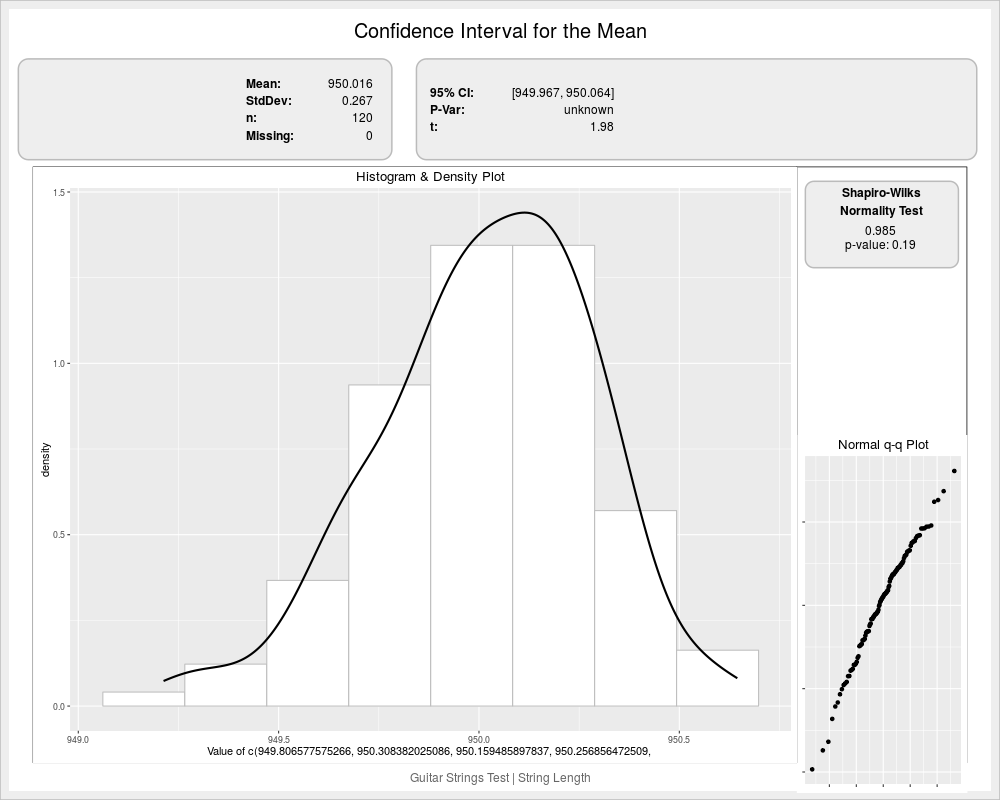
> example(ss.ci)
ss.ci> ss.ci(len, data=ss.data.strings, alpha = 0.05,
ss.ci+ sub = "Guitar Strings Test | String Length",
ss.ci+ xname = "Length")
Mean = 950.016; sd = 0.267
95% Confidence Interval= 949.967 to 950.064
LL UL
949.9674 950.0640
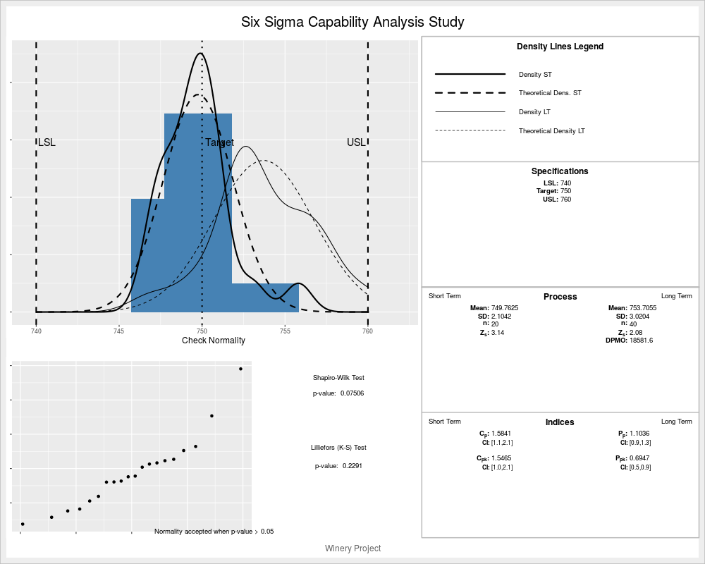
> example(ss.study.ca)
ss.st.> ss.study.ca(ss.data.ca$Volume, rnorm(40, 753, 3),
ss.st.+ LSL = 740, USL = 760, T = 750, alpha = 0.05,
ss.st.+ f.sub = "Winery Project")
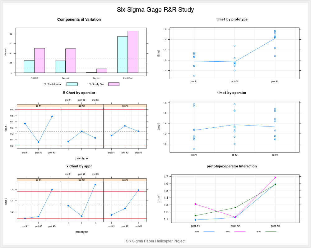
> example(ss.rr)
ss.rr> ss.rr(time1, prototype, operator, data = ss.data.rr,
ss.rr+ sub = "Six Sigma Paper Helicopter Project",
ss.rr+ alphaLim = 0.05,
ss.rr+ errorTerm = "interaction")
Complete model (with interaction):
Df Sum Sq Mean Sq F value Pr(>F)
prototype 2 1.2007 0.6004 28.797 0.00422
operator 2 0.0529 0.0265 1.270 0.37415
prototype:operator 4 0.0834 0.0208 0.974 0.44619
Repeatability 18 0.3854 0.0214
Total 26 1.7225
alpha for removing interaction: 0.05
Reduced model (without interaction):
Df Sum Sq Mean Sq F value Pr(>F)
prototype 2 1.2007 0.6004 28.174 8.56e-07
operator 2 0.0529 0.0265 1.242 0.308
Repeatability 22 0.4688 0.0213
Total 26 1.7225
Gage R&R
VarComp %Contrib
Total Gage R&R 0.0218823 25.38
Repeatability 0.0213088 24.71
Reproducibility 0.0005735 0.67
operator 0.0005735 0.67
Part-To-Part 0.0643389 74.62
Total Variation 0.0862212 100.00
StdDev StudyVar %StudyVar
Total Gage R&R 0.14792667 0.8875600 50.38
Repeatability 0.14597534 0.8758520 49.71
Reproducibility 0.02394786 0.1436872 8.16
operator 0.02394786 0.1436872 8.16
Part-To-Part 0.25365114 1.5219068 86.38
Total Variation 0.29363447 1.7618068 100.00
Number of Distinct Categories = 2
> example(ss.lf)
ss.lf> #Example bolts: evaluate LF at 10.5 if Target=10, Tolerance=0.5, L_0=0.001
ss.lf> ss.lf(10.5, 0.5, 10, 0.001)
[1] 5e-04
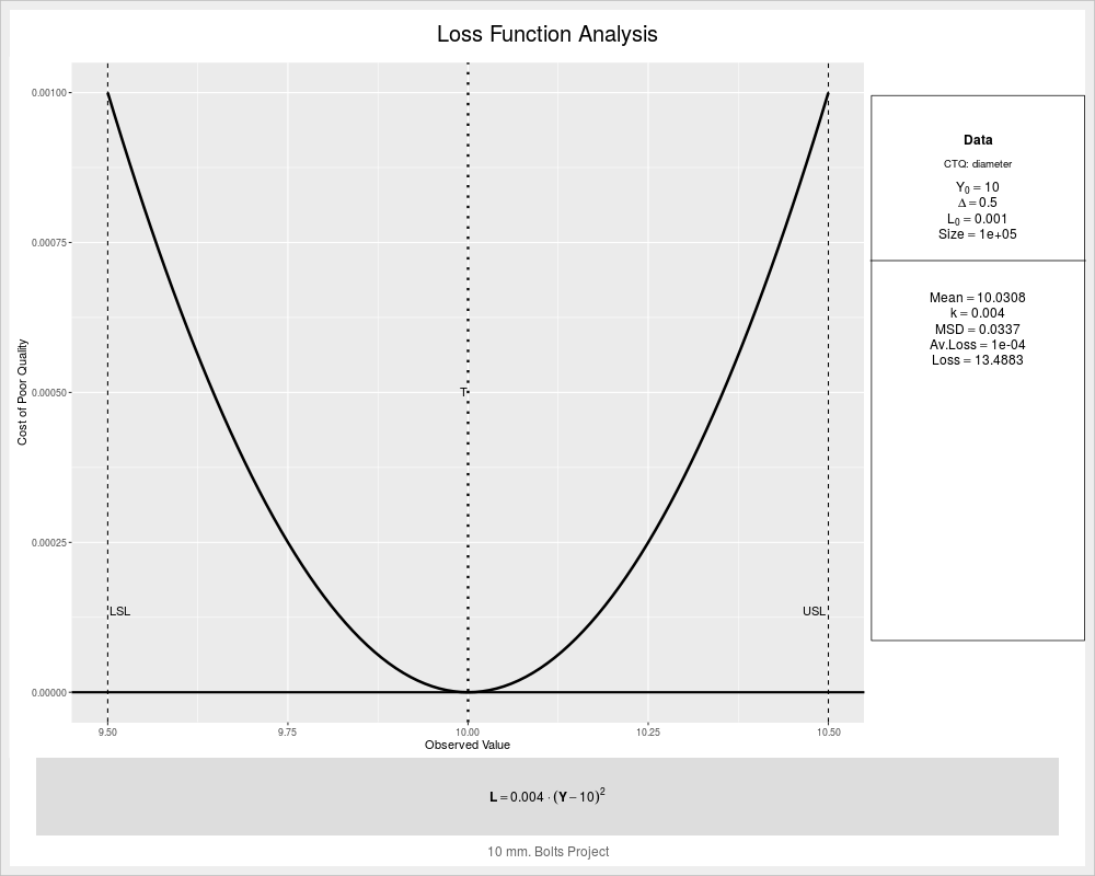
> example(ss.lfa)
ss.lfa> ss.lfa(ss.data.bolts, "diameter", 0.5, 10, 0.001,
ss.lfa+ lfa.sub = "10 mm. Bolts Project",
ss.lfa+ lfa.size = 100000, lfa.output = "both")
$lfa.k
[1] 0.004
$lfa.lf
expression(bold(L == 0.004 %.% (Y - 10)^2))
$lfa.MSD
[1] 0.03372065
$lfa.avLoss
[1] 0.0001348826
$lfa.Loss
[1] 13.48826
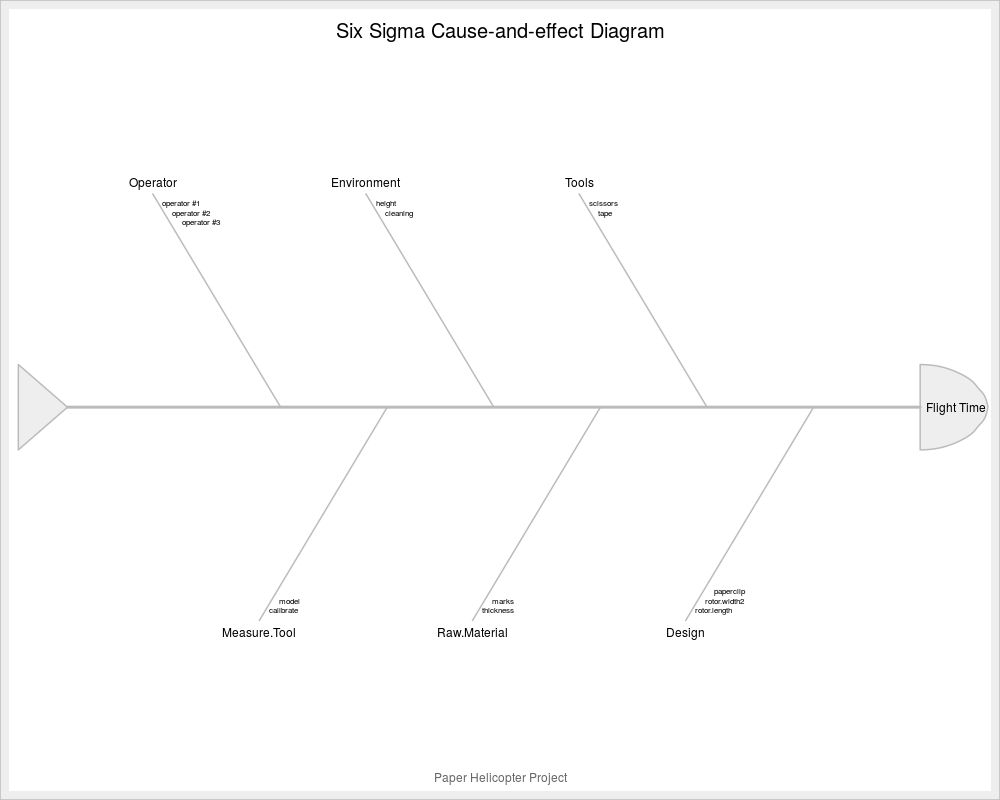
> example(ss.ceDiag)
ss.cDg> effect <- "Flight Time"
ss.cDg> causes.gr <- c("Operator", "Environment", "Tools", "Design",
ss.cDg+ "Raw.Material", "Measure.Tool")
ss.cDg> causes <- vector(mode = "list", length = length(causes.gr))
ss.cDg> causes[1] <- list(c("operator #1", "operator #2", "operator #3"))
ss.cDg> causes[2] <- list(c("height", "cleaning"))
ss.cDg> causes[3] <- list(c("scissors", "tape"))
ss.cDg> causes[4] <- list(c("rotor.length", "rotor.width2", "paperclip"))
ss.cDg> causes[5] <- list(c("thickness", "marks"))
ss.cDg> causes[6] <- list(c("calibrate", "model"))
ss.cDg> ss.ceDiag(effect, causes.gr, causes, sub = "Paper Helicopter Project")
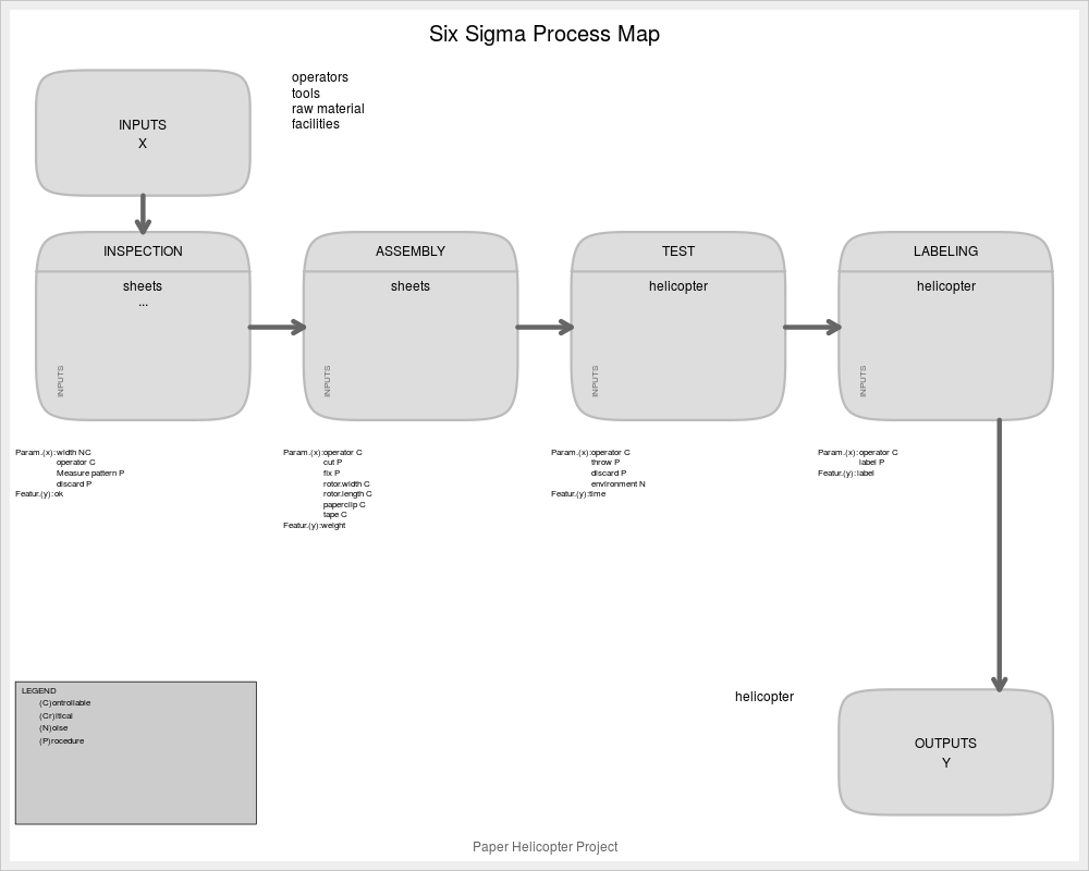
> example(ss.pMap)
ss.pMp> inputs.overall<-c("operators", "tools", "raw material", "facilities")
ss.pMp> outputs.overall<-c("helicopter")
ss.pMp> steps<-c("INSPECTION", "ASSEMBLY", "TEST", "LABELING")
ss.pMp> #Inputs of process "i" are inputs of process "i+1"
ss.pMp> input.output<-vector(mode="list",length=length(steps))
ss.pMp> input.output[1]<-list(c("sheets", "..."))
ss.pMp> input.output[2]<-list(c("sheets"))
ss.pMp> input.output[3]<-list(c("helicopter"))
ss.pMp> input.output[4]<-list(c("helicopter"))
ss.pMp> #Parameters of each process
ss.pMp> x.parameters<-vector(mode="list",length=length(steps))
ss.pMp> x.parameters[1]<-list(c(list(c("width", "NC")),list(c("operator", "C")),
ss.pMp+ list(c("Measure pattern", "P")), list(c("discard", "P"))))
ss.pMp> x.parameters[2]<-list(c(list(c("operator", "C")),list(c("cut", "P")),
ss.pMp+ list(c("fix", "P")), list(c("rotor.width", "C")),list(c("rotor.length",
ss.pMp+ "C")), list(c("paperclip", "C")), list(c("tape", "C"))))
ss.pMp> x.parameters[3]<-list(c(list(c("operator", "C")),list(c("throw", "P")),
ss.pMp+ list(c("discard", "P")), list(c("environment", "N"))))
ss.pMp> x.parameters[4]<-list(c(list(c("operator", "C")),list(c("label", "P"))))
ss.pMp> x.parameters
[[1]]
[[1]][[1]]
[1] "width" "NC"
[[1]][[2]]
[1] "operator" "C"
[[1]][[3]]
[1] "Measure pattern" "P"
[[1]][[4]]
[1] "discard" "P"
[[2]]
[[2]][[1]]
[1] "operator" "C"
[[2]][[2]]
[1] "cut" "P"
[[2]][[3]]
[1] "fix" "P"
[[2]][[4]]
[1] "rotor.width" "C"
[[2]][[5]]
[1] "rotor.length" "C"
[[2]][[6]]
[1] "paperclip" "C"
[[2]][[7]]
[1] "tape" "C"
[[3]]
[[3]][[1]]
[1] "operator" "C"
[[3]][[2]]
[1] "throw" "P"
[[3]][[3]]
[1] "discard" "P"
[[3]][[4]]
[1] "environment" "N"
[[4]]
[[4]][[1]]
[1] "operator" "C"
[[4]][[2]]
[1] "label" "P"
ss.pMp> #Features of each process
ss.pMp> y.features<-vector(mode="list",length=length(steps))
ss.pMp> y.features[1]<-list(c(list(c("ok", "Cr"))))
ss.pMp> y.features[2]<-list(c(list(c("weight", "Cr"))))
ss.pMp> y.features[3]<-list(c(list(c("time", "Cr"))))
ss.pMp> y.features[4]<-list(c(list(c("label", "Cr"))))
ss.pMp> y.features
[[1]]
[[1]][[1]]
[1] "ok" "Cr"
[[2]]
[[2]][[1]]
[1] "weight" "Cr"
[[3]]
[[3]][[1]]
[1] "time" "Cr"
[[4]]
[[4]][[1]]
[1] "label" "Cr"
ss.pMp> ss.pMap(steps, inputs.overall, outputs.overall,
ss.pMp+ input.output, x.parameters, y.features,
ss.pMp+ sub="Paper Helicopter Project")
> example(ss.ca.yield)
ss.c.y> ss.ca.yield(c(3,5,12),c(1,2,4),1915)
Yield FTY RTY DPU DPMO
1 0.9895561 0.9859008 0.9859563 20 10443.86
> example(ss.ca.z)
ss.c.z> ss.ca.cp(ss.data.ca$Volume,740, 760)
[1] 1.584136
ss.c.z> ss.ca.cpk(ss.data.ca$Volume,740, 760)
[1] 1.546513
ss.c.z> ss.ca.z(ss.data.ca$Volume,740,760)
[1] 3.139539
> example(ss.ca.cp)
ss.c.c> ss.ca.cp(ss.data.ca$Volume,740, 760)
[1] 1.584136
ss.c.c> ss.ca.cpk(ss.data.ca$Volume,740, 760)
[1] 1.546513
ss.c.c> ss.ca.z(ss.data.ca$Volume,740,760)
[1] 3.139539
> example(ss.ca.cpk)
ss.c.c> ss.ca.cp(ss.data.ca$Volume,740, 760)
[1] 1.584136
ss.c.c> ss.ca.cpk(ss.data.ca$Volume,740, 760)
[1] 1.546513
ss.c.c> ss.ca.z(ss.data.ca$Volume,740,760)
[1] 3.139539
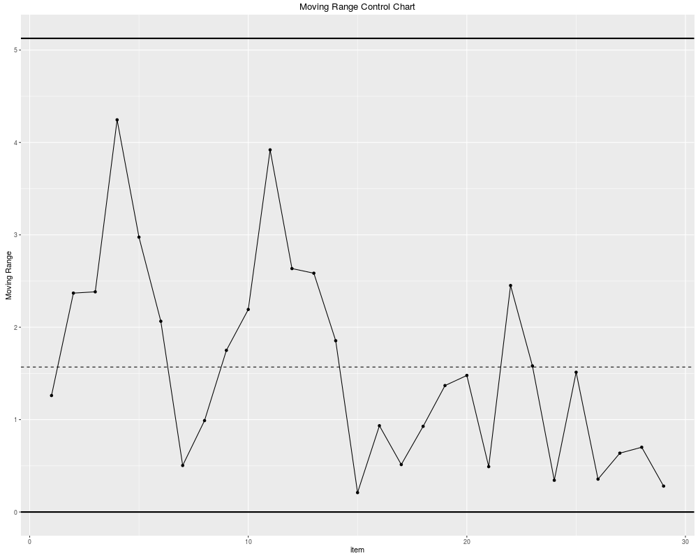
> example(ss.cc)
ss.cc> ss.cc("mr", ss.data.pb1, CTQ = "pb.humidity")
Phase I limits:
LCL CL UCL
0.000000 1.569483 5.126767
Out of control Moving Range:
None
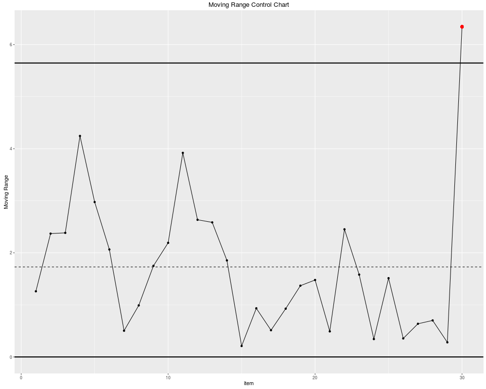
ss.cc> testout <- ss.data.pb1
ss.cc> testout[31,] <- list(31,17)
ss.cc> ss.cc("mr", testout, CTQ = "pb.humidity")
Phase I limits:
LCL CL UCL
0.000000 1.728600 5.646528
Out of control Moving Range:
[1] 30
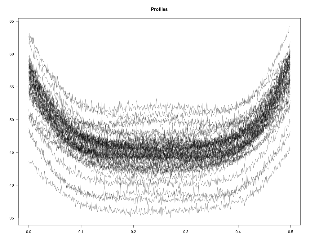
> example(plotProfiles)
pltPrf> plotProfiles(profiles = ss.data.wby,
pltPrf+ x = ss.data.wbx)
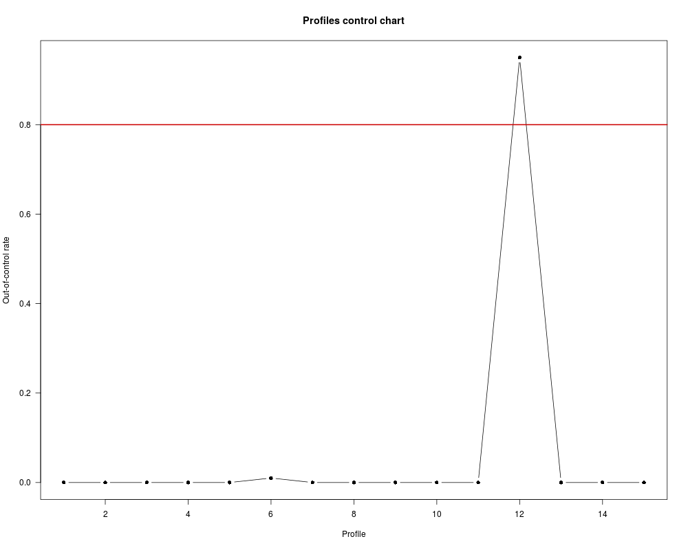
> example(plotControlProfiles)
pltCnP> wby.phase1 <- ss.data.wby[, 1:35]
pltCnP> wb.limits <- climProfiles(profiles = wby.phase1,
pltCnP+ x = ss.data.wbx,
pltCnP+ smoothprof = TRUE,
pltCnP+ smoothlim = TRUE)
pltCnP> wby.phase2 <- ss.data.wby[, 36:50]
pltCnP> wb.out.phase2 <- outProfiles(profiles = wby.phase2,
pltCnP+ x = ss.data.wbx,
pltCnP+ cLimits = wb.limits,
pltCnP+ tol = 0.8)
pltCnP> plotControlProfiles(wb.out.phase2$pOut, tol = 0.8)
>
>
>
>
>
> dev.off()
null device
1
>
|