## Load SplicingGraphs object 'TSPCsg':
filepath <- system.file("extdata", "TSPCsg.rda", package="SplicingGraphs")
load(filepath)
TSPCsg
## 'TSPCsg' has 1 element per gene and 'names(sg)' gives the gene ids.
names(TSPCsg)
## 1 splicing graph per gene. (Note that gene MUC16 was dropped
## because transcripts T-4 and T-5 in this gene both have their
## 2nd exon *inside* their 3rd exon. Splicing graph theory doesn't
## apply in that case.)
## Extract the edges of a given graph:
TSPCsgedges <- sgedges(TSPCsg["LGSN"])
TSPCsgedges
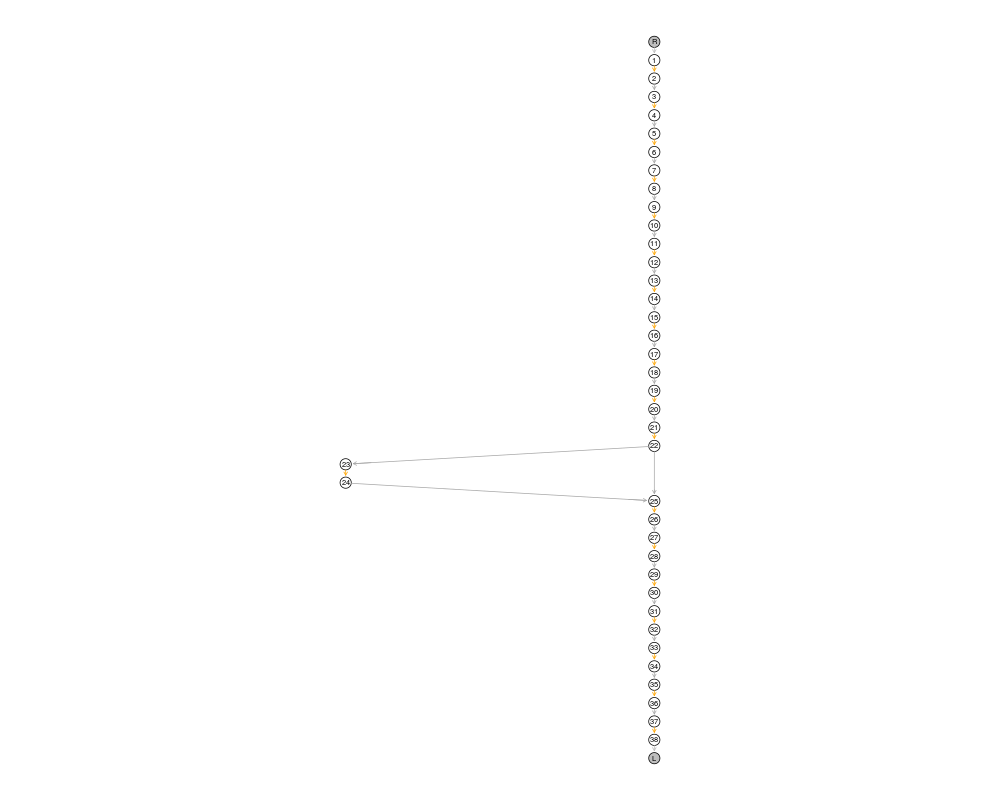
## Plot the graph for a given gene:
plot(TSPCsg["LGSN"]) # or 'plot(sgraph(TSPCsgedges))'
## The reads from all samples have been assigned to 'TSPCsg'.
## Use countReads() to summarize by splicing graph edge:
counts <- countReads(TSPCsg)
dim(counts)
counts[ , 1:5]
## You can subset 'TSPCsg' by 1 or more gene ids before calling
## countReads() in order to summarize only for those genes:
DAPL1counts <- countReads(TSPCsg["DAPL1"])
dim(DAPL1counts)
DAPL1counts[ , 1:5]
## Use 'by="rsgedge"' to summarize by *reduced* splicing graph edge:
DAPL1counts2 <- countReads(TSPCsg["DAPL1"], by="rsgedge")
dim(DAPL1counts2)
DAPL1counts2[ , 1:5]
## No reads assigned to genes KIAA0319L or TREM2 because no
## BAM files were provided for those genes:
KIAA0319Lcounts <- countReads(TSPCsg["KIAA0319L"])
KIAA0319Lcountsums <- sapply(KIAA0319Lcounts[ , -(1:2)], sum)
stopifnot(all(KIAA0319Lcountsums == 0))
TREM2counts <- countReads(TSPCsg["TREM2"])
TREM2countsums <- sapply(TREM2counts[ , -(1:2)], sum)
stopifnot(all(TREM2countsums == 0))
## Plot all the splicing graphs:
slideshow(TSPCsg)
Results
R version 3.3.1 (2016-06-21) -- "Bug in Your Hair"
Copyright (C) 2016 The R Foundation for Statistical Computing
Platform: x86_64-pc-linux-gnu (64-bit)

R is free software and comes with ABSOLUTELY NO WARRANTY.
You are welcome to redistribute it under certain conditions.
Type 'license()' or 'licence()' for distribution details.

R is a collaborative project with many contributors.
Type 'contributors()' for more information and
'citation()' on how to cite R or R packages in publications.

Type 'demo()' for some demos, 'help()' for on-line help, or
'help.start()' for an HTML browser interface to help.
Type 'q()' to quit R.

> library(SplicingGraphs)
Loading required package: GenomicFeatures
Loading required package: BiocGenerics
Loading required package: parallel

Attaching package: 'BiocGenerics'

The following objects are masked from 'package:parallel':

    clusterApply, clusterApplyLB, clusterCall, clusterEvalQ,
    clusterExport, clusterMap, parApply, parCapply, parLapply,
    parLapplyLB, parRapply, parSapply, parSapplyLB

The following objects are masked from 'package:stats':

    IQR, mad, xtabs

The following objects are masked from 'package:base':

    Filter, Find, Map, Position, Reduce, anyDuplicated, append,
    as.data.frame, cbind, colnames, do.call, duplicated, eval, evalq,
    get, grep, grepl, intersect, is.unsorted, lapply, lengths, mapply,
    match, mget, order, paste, pmax, pmax.int, pmin, pmin.int, rank,
    rbind, rownames, sapply, setdiff, sort, table, tapply, union,
    unique, unsplit

Loading required package: S4Vectors
Loading required package: stats4

Attaching package: 'S4Vectors'

The following objects are masked from 'package:base':

    colMeans, colSums, expand.grid, rowMeans, rowSums

Loading required package: IRanges
Loading required package: GenomeInfoDb
Loading required package: GenomicRanges
Loading required package: AnnotationDbi
Loading required package: Biobase
Welcome to Bioconductor

    Vignettes contain introductory material; view with
    'browseVignettes()'. To cite Bioconductor, see
    'citation("Biobase")', and for packages 'citation("pkgname")'.

Loading required package: GenomicAlignments
Loading required package: SummarizedExperiment
Loading required package: Biostrings
Loading required package: XVector
Loading required package: Rsamtools
Loading required package: Rgraphviz
Loading required package: graph

Attaching package: 'graph'

The following object is masked from 'package:Biostrings':

    complement

Loading required package: grid

Attaching package: 'Rgraphviz'

The following objects are masked from 'package:IRanges':

    from, to

The following objects are masked from 'package:S4Vectors':

    from, to

Warning messages:
1: replacing previous import 'IRanges::from' by 'Rgraphviz::from' when loading 'SplicingGraphs'
2: replacing previous import 'IRanges::to' by 'Rgraphviz::to' when loading 'SplicingGraphs'
> png(filename="/home/ddbj/snapshot/RGM3/R_BC/result/SplicingGraphs/TSPCsg.Rd_%03d_medium.png", width=480, height=480)
> ### Name: TSPCsg
> ### Title: TSPC splicing graphs
> ### Aliases: TSPCsg TSPC
>
> ### ** Examples
>
> ## Load SplicingGraphs object 'TSPCsg':
> filepath <- system.file("extdata", "TSPCsg.rda", package="SplicingGraphs")
> load(filepath)
> TSPCsg
SplicingGraphs object with 9 gene(s) and 33 transcript(s)
>
> ## 'TSPCsg' has 1 element per gene and 'names(sg)' gives the gene ids.
> names(TSPCsg)
[1] "BAI1"      "CYB561"    "DAPL1"     "ITGB8"     "KIAA0319L" "LGSN"
[7] "MKRN3"     "ST14"      "TREM2"
>
> ## 1 splicing graph per gene. (Note that gene MUC16 was dropped
> ## because transcripts T-4 and T-5 in this gene both have their
> ## 2nd exon *inside* their 3rd exon. Splicing graph theory doesn't
> ## apply in that case.)
>
> ## Extract the edges of a given graph:
> TSPCsgedges <- sgedges(TSPCsg["LGSN"])
> TSPCsgedges
DataFrame with 19 rows and 5 columns
           from          to   sgedge_id ex_or_in            tx_id
    <character> <character> <character> <factor>  <CharacterList>
1             R           1    LGSN:R,1           T-1,T-2,T-3,...
2             1           5    LGSN:1,5       ex         T-1,T-4n
3             5           6    LGSN:5,6       in T-1,T-2,T-4n,...
4             6           8    LGSN:6,8       ex T-1,T-2,T-4n,...
5             8          11   LGSN:8,11       in          T-1,T-2
...         ...         ...         ...      ...              ...
15            6           7    LGSN:6,7       ex              T-3
16            7           9    LGSN:7,9       in              T-3
17            9          10   LGSN:9,10       ex    T-3,T-4n,T-5n
18           10          11  LGSN:10,11       in    T-3,T-4n,T-5n
19            8           9    LGSN:8,9       in        T-4n,T-5n
>
> ## Plot the graph for a given gene:
> plot(TSPCsg["LGSN"])  # or 'plot(sgraph(TSPCsgedges))'
>
> ## The reads from all samples have been assigned to 'TSPCsg'.
> ## Use countReads() to summarize by splicing graph edge:
> counts <- countReads(TSPCsg)
> dim(counts)
[1] 249  56
> counts[ , 1:5]
DataFrame with 249 rows and 5 columns
      sgedge_id ex_or_in OVCAR3__OVCAR3 SOC_10764_474070 SOC_11199_480891
    <character> <factor>      <integer>        <integer>        <integer>
1      BAI1:1,2       ex              0                0                0
2      BAI1:2,3       in              0                0                0
3      BAI1:3,4       ex              0                0                0
4      BAI1:4,5       in              0                0                0
5      BAI1:5,6       ex              0                1                0
...         ...      ...            ...              ...              ...
245  TREM2:9,10       ex              0                0                0
246   TREM2:6,9       in              0                0                0
247   TREM2:2,3       in              0                0                0
248   TREM2:3,4       ex              0                0                0
249   TREM2:4,5       in              0                0                0
>
> ## You can subset 'TSPCsg' by 1 or more gene ids before calling
> ## countReads() in order to summarize only for those genes:
> DAPL1counts <- countReads(TSPCsg["DAPL1"])
> dim(DAPL1counts)
[1] 21 56
> DAPL1counts[ , 1:5]
DataFrame with 21 rows and 5 columns
      sgedge_id ex_or_in OVCAR3__OVCAR3 SOC_10764_474070 SOC_11199_480891
    <character> <factor>      <integer>        <integer>        <integer>
1     DAPL1:1,2       ex              2              757                4
2     DAPL1:2,3       in              1              296                1
3     DAPL1:3,4       ex              3             1040                8
4     DAPL1:4,5       in              2              451                7
5     DAPL1:5,6       ex              3              964               16
...         ...      ...            ...              ...              ...
17  DAPL1:18,19       ex              2                3                0
18    DAPL1:6,7       in              0               10                0
19    DAPL1:7,8       ex              0               10                0
20    DAPL1:8,9       in              0                0                0
21   DAPL1:6,17       in              0                0                0
>
> ## Use 'by="rsgedge"' to summarize by *reduced* splicing graph edge:
> DAPL1counts2 <- countReads(TSPCsg["DAPL1"], by="rsgedge")
> dim(DAPL1counts2)
[1] 11 56
> DAPL1counts2[ , 1:5]
DataFrame with 11 rows and 5 columns
         rsgedge_id ex_or_in OVCAR3__OVCAR3 SOC_10764_474070 SOC_11199_480891
        <character> <factor>      <integer>        <integer>        <integer>
1       DAPL1:1,2,3    mixed              2              757                4
2     DAPL1:3,4,5,6    mixed              4             1399               17
3         DAPL1:6,9       in              1              349                9
4        DAPL1:9,10       ex              1             1506               29
5     DAPL1:6,11,12    mixed              0               11                2
6    DAPL1:12,15,16    mixed              0                0                0
7  DAPL1:6,13,14,17    mixed              0                2                0
8       DAPL1:17,19       ex              2                3                0
9    DAPL1:12,18,19    mixed              2                3                0
10    DAPL1:6,7,8,9    mixed              0               10                0
11       DAPL1:6,17       in              0                0                0
>
> ## No reads assigned to genes KIAA0319L or TREM2 because no
> ## BAM files were provided for those genes:
> KIAA0319Lcounts <- countReads(TSPCsg["KIAA0319L"])
> KIAA0319Lcountsums <- sapply(KIAA0319Lcounts[ , -(1:2)], sum)
> stopifnot(all(KIAA0319Lcountsums == 0))
>
> TREM2counts <- countReads(TSPCsg["TREM2"])
> TREM2countsums <- sapply(TREM2counts[ , -(1:2)], sum)
> stopifnot(all(TREM2countsums == 0))
>
> ## Plot all the splicing graphs:
> slideshow(TSPCsg)
Plotting splicing graph for gene "BAI1" (2 transcript(s)). Press <Enter> for next...
Plotting splicing graph for gene "CYB561" (6 transcript(s)). Press <Enter> for next...
Plotting splicing graph for gene "DAPL1" (6 transcript(s)). Press <Enter> for next...
Plotting splicing graph for gene "ITGB8" (2 transcript(s)). Press <Enter> for next...
Plotting splicing graph for gene "KIAA0319L" (2 transcript(s)). Press <Enter> for next...
Plotting splicing graph for gene "LGSN" (5 transcript(s)). Press <Enter> for next...dev.off()
Plotting splicing graph for gene "MKRN3" (4 transcript(s)). Press <Enter> for next...Plotting splicing graph for gene "ST14" (2 transcript(s)). Press <Enter> for next...Plotting splicing graph for gene "TREM2" (4 transcript(s)). Press <Enter> for next...>
 .
.