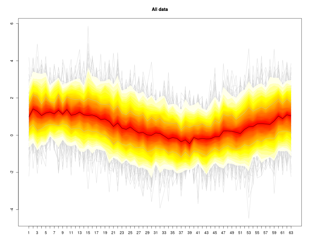
Visualization of a set of “profiles” (i.e. a consecutive series of measurements like a time series, or the DNA binding levels along different positions on a gene). The profiles are given as the rows of a (samples x positions) matrix that contains the measurements.
Instead of plotting a line for each profile (row of the matrix), the q-quantiles for each position (column of the matrix) are calculated, where q runs through a set of representative quantiles.
Then for each q, a line of q-quantiles is plotted along the positions. Color coding of the quantile profiles aids the interpretation of the plot: There is a color gradient from the median profile to the 0 (=min) resp. 1(=max) quantile.
a (samples x columns) matrix with numerical entries. Each sample row is understood as a consecutive series of measurements. Missing values are not allowed so far
label
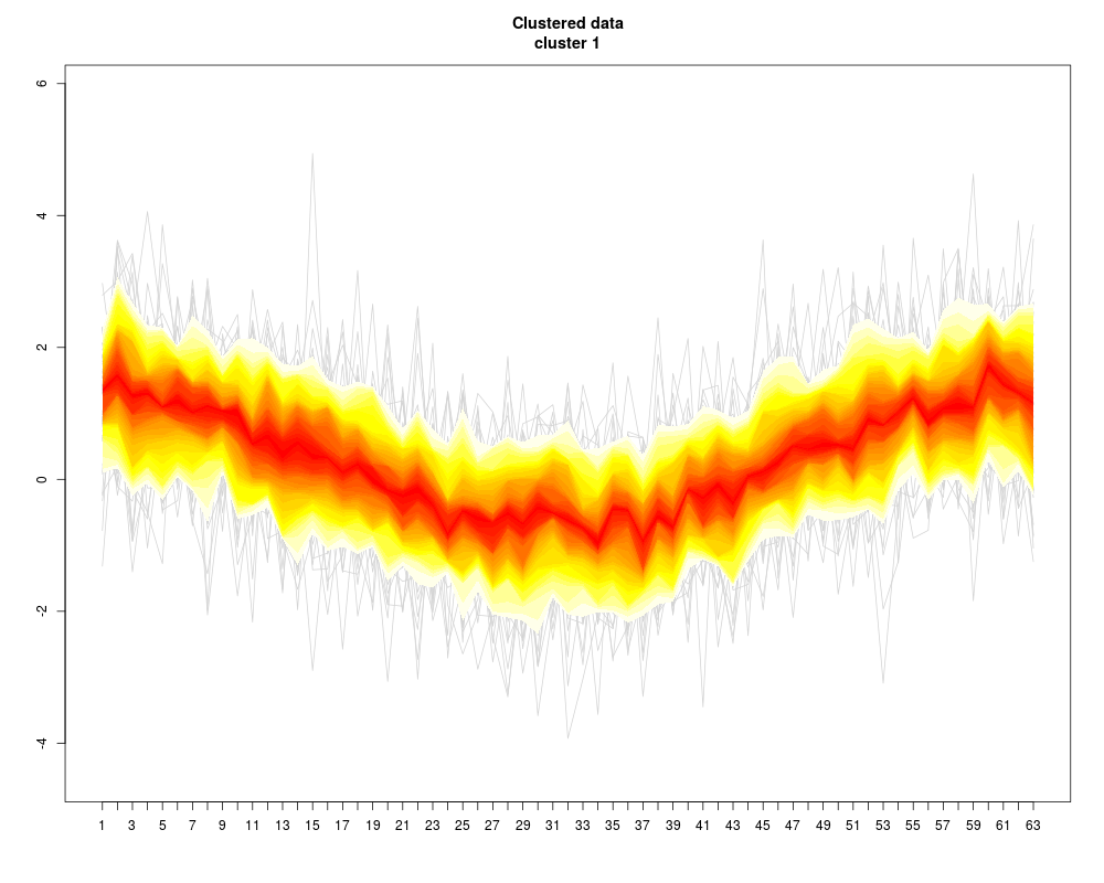
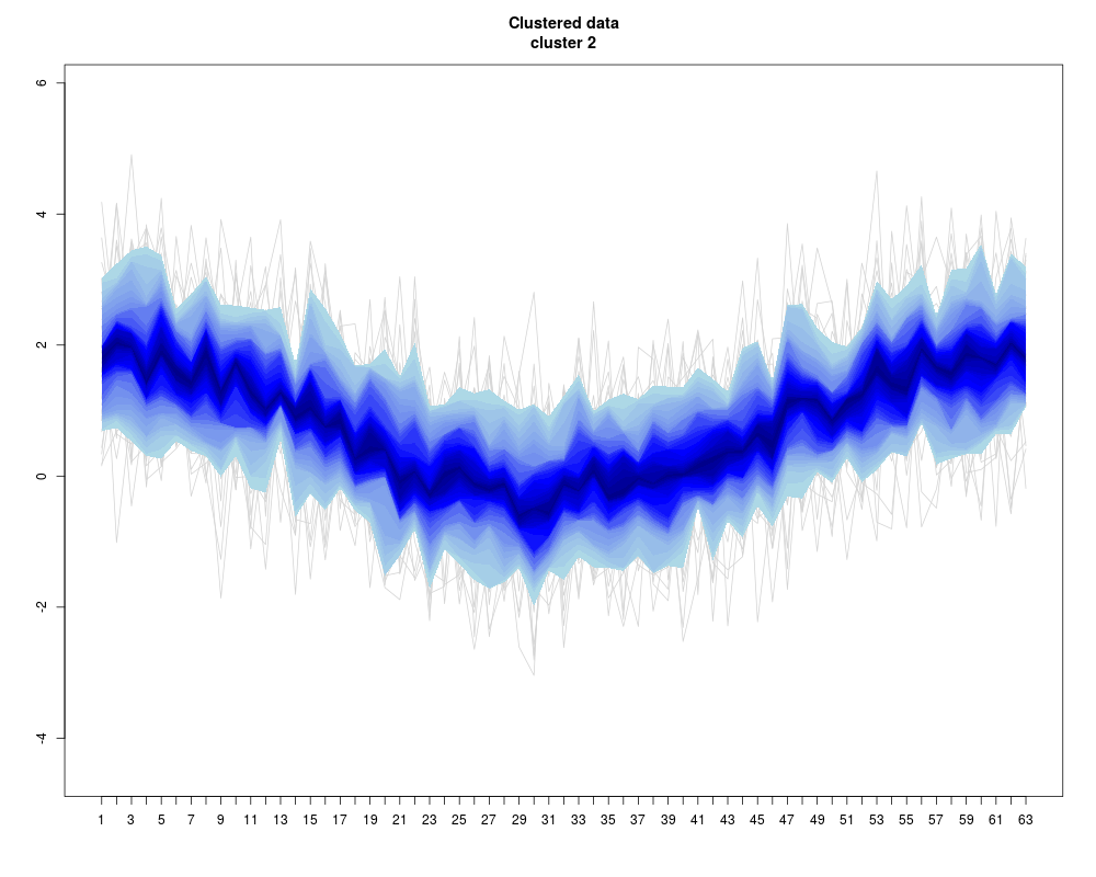
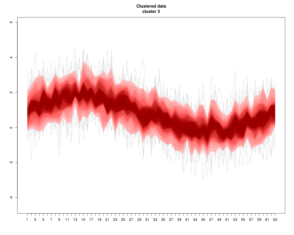
if multiple clusters should be plotted in one diagram, the cluster labels for each item are given in this vector
at
optional vector of length ncol(cluster), default = 1:ncol(cluster). Specifies the x-values at which the positions will be plotted.
main
the title of the plot, standard graphics parameter
xlim
xlimits, standard graphics parameter
xlab
x-axis legend, standard graphics parameter
xaxt
should an x axis be plotted at all? (="n" if not), standard graphics parameter
xlabels
character vector. If specified, this text will be added at the “at“-positions as x-axis labels.
las
direction of the xlabels text. las=1: horizontal text, las=2: vertical text
ylim
ylimits, standard graphics parameter
ylab
y-axis legend, standard graphics parameter
fromto
determines the smallest and the largest quantile that are plotted in colors, more distant values are plotted as outliers
colpal
either "red","green","blue" (predefined standard color palettes in profileplot), or a vector of colors to be used instead.
nrcolors
not very important. How many colors will the color palette contain? Usually, the default = 25 is sufficient
outer.col
color of the outlier lines, default = "light grey". For no outliers, choose outer.col="none"
add.quartiles
should the quartile lines be plotted (grey/black)? default=TRUE
add
should the profile plot be added to the current plot? Defaults to FALSE
separate
should each cluster, be plotted in a separate window? Defaults to TRUE
sampls = 100
probes = 63
at = (-31:31)*14
clus = matrix(rnorm(probes*sampls,sd=1),ncol=probes)
clus= rbind( t(t(clus)+sin(1:probes/10))+1:nrow(clus)/sampls , t(t(clus)+sin(pi/2+1:probes/10))+1:nrow(clus)/sampls )
labs = paste("cluster",kmeans(clus,4)$cluster)
profileplot(clus,main="All data",fromto=c(0,1))
profileplot(clus,label=labs,main="Clustered data",colpal=c("heat","blue","red","topo"),add.quartiles=FALSE)
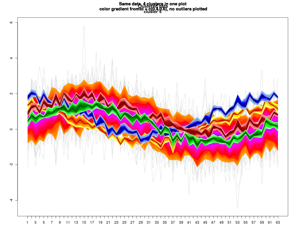
profileplot(clus,main="Same data, 4 clusters in one plot\n color gradient fromto = c(0.4,0.6), no outliers plotted",label=labs,separate=FALSE,xaxt="n",fromto=c(0.4,0.6),
colpal=c("heat","blue","red","green"),outer.col="none")
Results
R version 3.3.1 (2016-06-21) -- "Bug in Your Hair"
Copyright (C) 2016 The R Foundation for Statistical Computing
Platform: x86_64-pc-linux-gnu (64-bit)

R is free software and comes with ABSOLUTELY NO WARRANTY.
You are welcome to redistribute it under certain conditions.
Type 'license()' or 'licence()' for distribution details.

R is a collaborative project with many contributors.
Type 'contributors()' for more information and
'citation()' on how to cite R or R packages in publications.

Type 'demo()' for some demos, 'help()' for on-line help, or
'help.start()' for an HTML browser interface to help.
Type 'q()' to quit R.

> library(Starr)
Loading required package: Ringo
Loading required package: Biobase
Loading required package: BiocGenerics
Loading required package: parallel

Attaching package: 'BiocGenerics'

The following objects are masked from 'package:parallel':

    clusterApply, clusterApplyLB, clusterCall, clusterEvalQ,
    clusterExport, clusterMap, parApply, parCapply, parLapply,
    parLapplyLB, parRapply, parSapply, parSapplyLB

The following objects are masked from 'package:stats':

    IQR, mad, xtabs

The following objects are masked from 'package:base':

    Filter, Find, Map, Position, Reduce, anyDuplicated, append,
    as.data.frame, cbind, colnames, do.call, duplicated, eval, evalq,
    get, grep, grepl, intersect, is.unsorted, lapply, lengths, mapply,
    match, mget, order, paste, pmax, pmax.int, pmin, pmin.int, rank,
    rbind, rownames, sapply, setdiff, sort, table, tapply, union,
    unique, unsplit

Welcome to Bioconductor

    Vignettes contain introductory material; view with
    'browseVignettes()'. To cite Bioconductor, see
    'citation("Biobase")', and for packages 'citation("pkgname")'.

Loading required package: RColorBrewer
Loading required package: limma

Attaching package: 'limma'

The following object is masked from 'package:BiocGenerics':

    plotMA

Loading required package: Matrix
Loading required package: grid
Loading required package: lattice
Loading required package: affy

Attaching package: 'affy'

The following object is masked from 'package:Ringo':

    probes

Loading required package: affxparser

Attaching package: 'Starr'

The following object is masked from 'package:affy':

    plotDensity

The following object is masked from 'package:limma':

    plotMA

The following object is masked from 'package:BiocGenerics':

    plotMA

> png(filename="/home/ddbj/snapshot/RGM3/R_BC/result/Starr/profileplot.Rd_%03d_medium.png", width=480, height=480)
> ### Name: profileplot
> ### Title: Vizualize clusters
> ### Aliases: profileplot
> ### Keywords: hplot
>
> ### ** Examples
>
> sampls = 100
> probes = 63
> at = (-31:31)*14
> clus = matrix(rnorm(probes*sampls,sd=1),ncol=probes)
> clus= rbind( t(t(clus)+sin(1:probes/10))+1:nrow(clus)/sampls , t(t(clus)+sin(pi/2+1:probes/10))+1:nrow(clus)/sampls )
> labs = paste("cluster",kmeans(clus,4)$cluster)
>
> profileplot(clus,main="All data",fromto=c(0,1))
> profileplot(clus,label=labs,main="Clustered data",colpal=c("heat","blue","red","topo"),add.quartiles=FALSE)
> profileplot(clus,main="Same data, 4 clusters in one plot\n color gradient fromto = c(0.4,0.6), no outliers plotted",label=labs,separate=FALSE,xaxt="n",fromto=c(0.4,0.6),
+ 	colpal=c("heat","blue","red","green"),outer.col="none")
>
>
>
>
>
> dev.off()
null device
          1
>
 .
.