R Graphical Manual

Browse All

Last data update: 2014.03.03

R: Plot a log fold-change versus log average expression...

plot	R Documentation

Plot a log fold-change versus log average expression (so-called M-A plot)

Description

This function generates a scatter plot of log fold-change (i.e., M = log2(G2) - log2(G1) on the y-axis between Groups 1 vs. 2) versus log average expression (i.e., A = (log2(G1) + log2(G2)) / 2 on the x-axis) using normalized count data.

Usage

## S3 method for class 'TCC'
plot(x, FDR = NULL, median.lines = FALSE, floor = 0,
     group = NULL, col = NULL, col.tag = NULL, normalize = TRUE, ...)

Arguments

`x`	TCC-class object.
`FDR`	numeric scalar specifying a false discovery rate (FDR) threshold for determining differentially expressed genes (DEGs)
`median.lines`	logical. If `TRUE`, horizontal lines specifying the median M values for non-DEGs (black) and DEGs (red) are drawn.
`floor`	numeric scalar specifying a threshold for adjusting low count data.
`group`	numeric vector consists two elements for specifying what two groups should be drawn when data contains more than three groups.
`col`	vector specifying plotting color.
`col.tag`	numeric vector spacifying the index of `col` for coloring the points of the genes.
`normalize`	logical. If `FALSE`, the coordinates of M-A plot are calculated from the raw data.
`...`	further graphical arguments, see `plot.default`.

Details

This function generates roughly three different M-A plots depending on the conditions for TCC-class objects. When the function is performed just after the new method, all the genes (points) are treated as non-DEGs (the default is black; see Example 1). The simulateReadCounts function followed by the plot function can classify the genes as true non-DEGs (black), true DEGs. (see Example 2). The estimateDE function followed by the plot function generates estimated DEGs (magenta) and the remaining estimated non-DEGs (black).

Genes with normalized counts of 0 in any one group cannot be plotted on the M-A plot because those M and A values cannot be calculated (as log 0 is undefined). Those points are plotted at the left side of the M-A plot, depending on the minimum A (i.e., log average expression) value. The x coordinate of those points is the minimum A value minus one. The y coordinate is calculated as if the zero count was the minimum observed non zero count in each group.

Value

A scatter plot to the current graphic device.

Examples

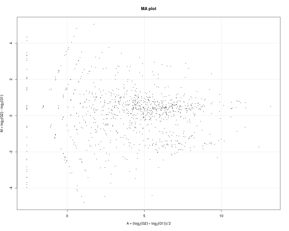
# Example 1. 
# M-A plotting just after constructing the TCC class object from
# hypoData. In this case, the plot is generated from hypoData
# that has been scaled in such a way that the library sizes of 
# each sample are the same as the mean library size of the
# original hypoData. Note that all points are in black. This is
# because the information about DEG or non-DEG for each gene is 
# not indicated.
data(hypoData)
group <- c(1, 1, 1, 2, 2, 2)
tcc <- new("TCC", hypoData, group)
plot(tcc)

normalized.count <- getNormalizedData(tcc)
colSums(normalized.count)
colSums(hypoData)
mean(colSums(hypoData))


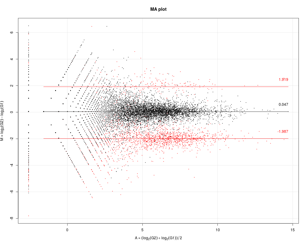
# Example 2. 
# M-A plotting of DEGES/edgeR-normalized simulation data.
# It can be seen that the median M value for non-DEGs approaches
# zero. Note that non-DEGs are in black, DEGs are in red.
tcc <- simulateReadCounts()
tcc <- calcNormFactors(tcc, norm.method = "tmm", test.method = "edger",
                       iteration = 1, FDR = 0.1, floorPDEG = 0.05)
plot(tcc, median.lines = TRUE)


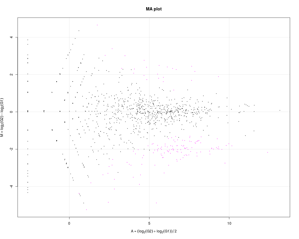
# Example 3. 
# M-A plotting of DEGES/edgeR-normalized hypoData after performing
# DE analysis.
data(hypoData)
group <- c(1, 1, 1, 2, 2, 2)
tcc <- new("TCC", hypoData, group)
tcc <- calcNormFactors(tcc, norm.method = "tmm", test.method = "edger",
                       iteration = 1, FDR = 0.1, floorPDEG = 0.05)
tcc <- estimateDE(tcc, test.method = "edger", FDR = 0.1)
plot(tcc)

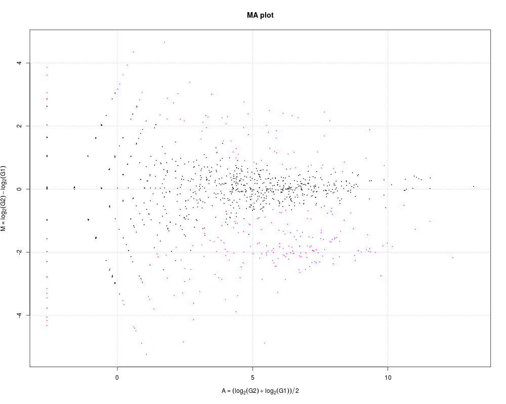
# Changing the FDR threshold
plot(tcc, FDR = 0.7)

Results


R version 3.3.1 (2016-06-21) -- "Bug in Your Hair"
Copyright (C) 2016 The R Foundation for Statistical Computing
Platform: x86_64-pc-linux-gnu (64-bit)

R is free software and comes with ABSOLUTELY NO WARRANTY.
You are welcome to redistribute it under certain conditions.
Type 'license()' or 'licence()' for distribution details.

R is a collaborative project with many contributors.
Type 'contributors()' for more information and
'citation()' on how to cite R or R packages in publications.

Type 'demo()' for some demos, 'help()' for on-line help, or
'help.start()' for an HTML browser interface to help.
Type 'q()' to quit R.

> library(TCC)
Loading required package: DESeq
Loading required package: BiocGenerics
Loading required package: parallel

Attaching package: 'BiocGenerics'

The following objects are masked from 'package:parallel':

    clusterApply, clusterApplyLB, clusterCall, clusterEvalQ,
    clusterExport, clusterMap, parApply, parCapply, parLapply,
    parLapplyLB, parRapply, parSapply, parSapplyLB

The following objects are masked from 'package:stats':

    IQR, mad, xtabs

The following objects are masked from 'package:base':

    Filter, Find, Map, Position, Reduce, anyDuplicated, append,
    as.data.frame, cbind, colnames, do.call, duplicated, eval, evalq,
    get, grep, grepl, intersect, is.unsorted, lapply, lengths, mapply,
    match, mget, order, paste, pmax, pmax.int, pmin, pmin.int, rank,
    rbind, rownames, sapply, setdiff, sort, table, tapply, union,
    unique, unsplit

Loading required package: Biobase
Welcome to Bioconductor

    Vignettes contain introductory material; view with
    'browseVignettes()'. To cite Bioconductor, see
    'citation("Biobase")', and for packages 'citation("pkgname")'.

Loading required package: locfit
locfit 1.5-9.1 	 2013-03-22
Loading required package: lattice
    Welcome to 'DESeq'. For improved performance, usability and
    functionality, please consider migrating to 'DESeq2'.
Loading required package: DESeq2
Loading required package: S4Vectors
Loading required package: stats4

Attaching package: 'S4Vectors'

The following objects are masked from 'package:base':

    colMeans, colSums, expand.grid, rowMeans, rowSums

Loading required package: IRanges
Loading required package: GenomicRanges
Loading required package: GenomeInfoDb
Loading required package: SummarizedExperiment

Attaching package: 'DESeq2'

The following objects are masked from 'package:DESeq':

    estimateSizeFactorsForMatrix, getVarianceStabilizedData,
    varianceStabilizingTransformation

Loading required package: edgeR
Loading required package: limma

Attaching package: 'limma'

The following object is masked from 'package:DESeq2':

    plotMA

The following object is masked from 'package:DESeq':

    plotMA

The following object is masked from 'package:BiocGenerics':

    plotMA

Loading required package: baySeq
Loading required package: abind
Loading required package: perm
Loading required package: ROC

Attaching package: 'TCC'

The following object is masked from 'package:edgeR':

    calcNormFactors

> png(filename="/home/ddbj/snapshot/RGM3/R_BC/result/TCC/plot.TCC.Rd_%03d_medium.png", width=480, height=480)
> ### Name: plot
> ### Title: Plot a log fold-change versus log average expression (so-called
> ###   M-A plot)
> ### Aliases: plot.TCC plot
> ### Keywords: methods
> 
> ### ** Examples
> 
> # Example 1. 
> # M-A plotting just after constructing the TCC class object from
> # hypoData. In this case, the plot is generated from hypoData
> # that has been scaled in such a way that the library sizes of 
> # each sample are the same as the mean library size of the
> # original hypoData. Note that all points are in black. This is
> # because the information about DEG or non-DEG for each gene is 
> # not indicated.
> data(hypoData)
> group <- c(1, 1, 1, 2, 2, 2)
> tcc <- new("TCC", hypoData, group)
> plot(tcc)
> 
> normalized.count <- getNormalizedData(tcc)
> colSums(normalized.count)
 G1_rep1  G1_rep2  G1_rep3  G2_rep1  G2_rep2  G2_rep3 
125922.3 125922.3 125922.3 125922.3 125922.3 125922.3 
> colSums(hypoData)
G1_rep1 G1_rep2 G1_rep3 G2_rep1 G2_rep2 G2_rep3 
 142177  145289  149886  112100  104107  101975 
> mean(colSums(hypoData))
[1] 125922.3
> 
> 
> # Example 2. 
> # M-A plotting of DEGES/edgeR-normalized simulation data.
> # It can be seen that the median M value for non-DEGs approaches
> # zero. Note that non-DEGs are in black, DEGs are in red.
> tcc <- simulateReadCounts()
TCC::INFO: Generating simulation data under NB distribution ...
TCC::INFO: (genesizes   :  10000 )
TCC::INFO: (replicates  :  3, 3 )
TCC::INFO: (PDEG        :  0.18, 0.02 )
> tcc <- calcNormFactors(tcc, norm.method = "tmm", test.method = "edger",
+                        iteration = 1, FDR = 0.1, floorPDEG = 0.05)
TCC::INFO: Calculating normalization factors using DEGES
TCC::INFO: (iDEGES pipeline : tmm - [ edger - tmm ] X 1 )
TCC::INFO: Done.
> plot(tcc, median.lines = TRUE)
> 
> 
> # Example 3. 
> # M-A plotting of DEGES/edgeR-normalized hypoData after performing
> # DE analysis.
> data(hypoData)
> group <- c(1, 1, 1, 2, 2, 2)
> tcc <- new("TCC", hypoData, group)
> tcc <- calcNormFactors(tcc, norm.method = "tmm", test.method = "edger",
+                        iteration = 1, FDR = 0.1, floorPDEG = 0.05)
TCC::INFO: Calculating normalization factors using DEGES
TCC::INFO: (iDEGES pipeline : tmm - [ edger - tmm ] X 1 )
TCC::INFO: Done.
> tcc <- estimateDE(tcc, test.method = "edger", FDR = 0.1)
TCC::INFO: Identifying DE genes using edger ...
TCC::INFO: Done.
> plot(tcc)
> 
> # Changing the FDR threshold
> plot(tcc, FDR = 0.7)
> 
> 
> 
> 
> 
> dev.off()
null device 
          1 
>