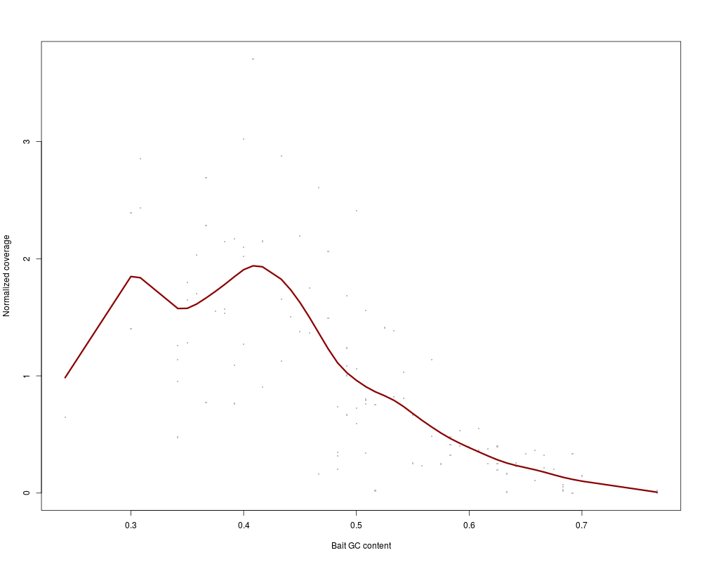
Bait coverage versus GC content plot

Description

Calculates and plots average normalized coverage per hybridization probe versus GC content of the respective probe. A smoothing spline is added to the scatter plot.

Usage

coverage.GC(coverageAll, baits, returnBaitValues = FALSE, linecol = "darkred", lwd, xlab, ylab, pch, col, cex, ...)

Arguments

Details

The function calculates average normalized coverages for each bait: the average coverage over all bases within a bait is divided by the average coverage over all bait-covered bases. Normalized coverages are not dependent on the absolute quantity of reads and are hence better comparable between different samples or even different experiments.

Value

A scatterplot with normalized per-bait coverages on the y-axis and GC content of respective baits on the x-axis. A smoothing spline is added to the plot.

If returnBaitValues = TRUE average coverage, average normalized coverage and GC content per bait are returned as 'values' columns of the baits input RangedData table

Author(s)

Manuela Hummel m.hummel@dkfz.de

References

Tewhey R, Nakano M, Wang X, Pabon-Pena C, Novak B, Giuffre A, Lin E, Happe S, Roberts DN, LeProust EM, Topol EJ, Harismendy O, Frazer KA. Enrichment of sequencing targets from the human genome by solution hybridization. Genome Biol. 2009; 10(10): R116.

See Also

coverage.target, covered.k, coverage.hist, coverage.plot, coverage.uniformity, coverage.targetlength.plot

Examples

## get reads and targets
exptPath <- system.file("extdata", package="TEQC")
readsfile <- file.path(exptPath, "ExampleSet_Reads.bed")
reads <- get.reads(readsfile, idcol=4, skip=0)
targetsfile <- file.path(exptPath, "ExampleSet_Targets.bed")
targets <- get.targets(targetsfile, skip=0)

## calculate per-base coverages
Coverage <- coverage.target(reads, targets, perBase=TRUE)

## get bait positions and sequences
baitsfile <- file.path(exptPath, "ExampleSet_Baits.txt")
baits <- get.baits(baitsfile, chrcol=3, startcol=4, endcol=5, seqcol=2)

## do coverage vs GC plot
coverage.GC(Coverage$coverageAll, baits)

Results

R version 3.3.1 (2016-06-21) -- "Bug in Your Hair"
Copyright (C) 2016 The R Foundation for Statistical Computing
Platform: x86_64-pc-linux-gnu (64-bit)

R is free software and comes with ABSOLUTELY NO WARRANTY.
You are welcome to redistribute it under certain conditions.
Type 'license()' or 'licence()' for distribution details.

R is a collaborative project with many contributors.
Type 'contributors()' for more information and
'citation()' on how to cite R or R packages in publications.

Type 'demo()' for some demos, 'help()' for on-line help, or
'help.start()' for an HTML browser interface to help.
Type 'q()' to quit R.

> library(TEQC)
Loading required package: BiocGenerics
Loading required package: parallel

Attaching package: 'BiocGenerics'

The following objects are masked from 'package:parallel':

    clusterApply, clusterApplyLB, clusterCall, clusterEvalQ,
    clusterExport, clusterMap, parApply, parCapply, parLapply,
    parLapplyLB, parRapply, parSapply, parSapplyLB

The following objects are masked from 'package:stats':

    IQR, mad, xtabs

The following objects are masked from 'package:base':

    Filter, Find, Map, Position, Reduce, anyDuplicated, append,
    as.data.frame, cbind, colnames, do.call, duplicated, eval, evalq,
    get, grep, grepl, intersect, is.unsorted, lapply, lengths, mapply,
    match, mget, order, paste, pmax, pmax.int, pmin, pmin.int, rank,
    rbind, rownames, sapply, setdiff, sort, table, tapply, union,
    unique, unsplit

Loading required package: IRanges
Loading required package: S4Vectors
Loading required package: stats4

Attaching package: 'S4Vectors'

The following objects are masked from 'package:base':

    colMeans, colSums, expand.grid, rowMeans, rowSums

Loading required package: Rsamtools
Loading required package: GenomeInfoDb
Loading required package: GenomicRanges
Loading required package: Biostrings
Loading required package: XVector
Loading required package: hwriter
> png(filename="/home/ddbj/snapshot/RGM3/R_BC/result/TEQC/coverage.GC.Rd_%03d_medium.png", width=480, height=480)
> ### Name: coverage.GC
> ### Title: Bait coverage versus GC content plot
> ### Aliases: coverage.GC
> ### Keywords: hplot
> 
> ### ** Examples
> 
> ## get reads and targets
> exptPath <- system.file("extdata", package="TEQC")
> readsfile <- file.path(exptPath, "ExampleSet_Reads.bed")
> reads <- get.reads(readsfile, idcol=4, skip=0)
[1] "read 19546 sequenced reads"
> targetsfile <- file.path(exptPath, "ExampleSet_Targets.bed")
> targets <- get.targets(targetsfile, skip=0)
[1] "read 50 (non-overlapping) target regions"
Warning message:
the "reduce" method for RangedData object is deprecated 
> 
> ## calculate per-base coverages
> Coverage <- coverage.target(reads, targets, perBase=TRUE)
> 
> ## get bait positions and sequences
> baitsfile <- file.path(exptPath, "ExampleSet_Baits.txt")
> baits <- get.baits(baitsfile, chrcol=3, startcol=4, endcol=5, seqcol=2)
[1] "read 108 hybridization probes"
> 
> ## do coverage vs GC plot
> coverage.GC(Coverage$coverageAll, baits)
> 
> 
> 
> 
> 
> dev.off()
null device 
          1 
>