R Graphical Manual

Browse All

Last data update: 2014.03.03

R: Coverage correlation plot

coverage.correlation

R Documentation

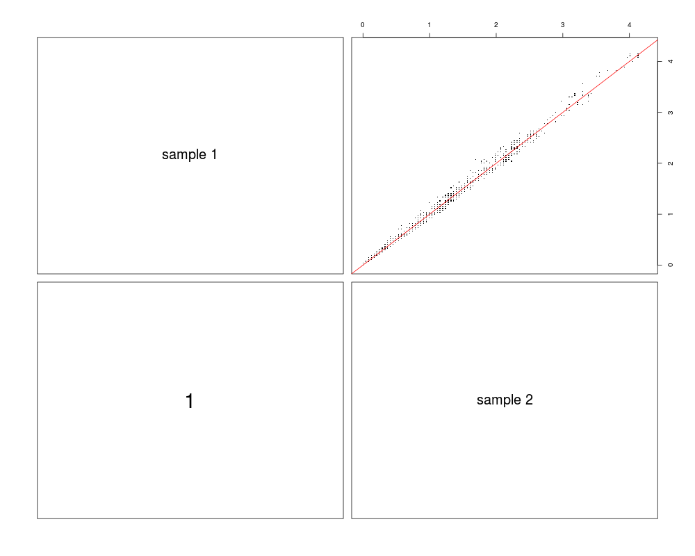
Coverage correlation plot

Description

Visualization of target coverage correlations between pairs of samples.

Usage

coverage.correlation(coveragelist, normalized = TRUE, plotfrac = 0.001, seed = 123, labels, main, pch = ".", cex.labels,
                  cex.pch = 2, cex.main = 1.2, cex.corr, font.labels = 1, font.main = 2, ...)

Arguments

`coveragelist`	List where each element is the output of function `coverage.target`, where option `perBase` had to be set to `TRUE`.
`normalized`	if `TRUE`, correlation of normalized target coverages will be shown; original coverages otherwise
`plotfrac`	numeric value between 0 and 1. Coverages for a fraction of `plotfrac` of all target bases are shown.
`seed`	seed for random selection of `plotfrac` bases
`labels`	sample names that are written in the diagonal panels; if missing, names of `coveragelist` are taken; if those are `NULL`, "sample 'i'" is shown
`main`	main title
`pch`	plot symbol for the scatter plots
`cex.labels, cex.pch, cex.main`	sizes of sample labels, plot symbols, main title
`cex.corr`	size of the correlation values; if missing, sizes are made proportionally to the values of (positive) correlation.
`font.labels, font.main`	fonts for sample labels and main title
`...`	further graphical parameters, e.g. limits and symbol color for the scatter plots

Details

If normalized = TRUE, the function calculates normalized coverages: per-base coverages divided by average coverage over all targeted bases. Normalized coverages are not dependent on the absolute quantity of reads and are hence better comparable between different samples or even different experiments.

Value

'pairs'-style plot where upper panels show scatter plot of (a randomly chosen fraction of) coverage values for pairs of samples. The lower panels show the respective Pearson correlation coefficients, calculated using all coverage values (even if not all of them are shown in the scatter plot).

Author(s)

Manuela Hummel m.hummel@dkfz.de

Examples

## get reads and targets
exptPath <- system.file("extdata", package="TEQC")
readsfile <- file.path(exptPath, "ExampleSet_Reads.bed")
reads <- get.reads(readsfile, idcol=4, skip=0)
targetsfile <- file.path(exptPath, "ExampleSet_Targets.bed")
targets <- get.targets(targetsfile, skip=0)

## calculate per-base coverages
Coverage <- coverage.target(reads, targets, perBase=TRUE)

## simulate another sample
r <- sample(nrow(reads), 0.1 * nrow(reads))
reads2 <- reads[-r,,drop=TRUE]
Coverage2 <- coverage.target(reads2, targets, perBase=TRUE)

## coverage uniformity plot
covlist <- list(Coverage, Coverage2)
coverage.correlation(covlist, plotfrac=0.1)

Results


R version 3.3.1 (2016-06-21) -- "Bug in Your Hair"
Copyright (C) 2016 The R Foundation for Statistical Computing
Platform: x86_64-pc-linux-gnu (64-bit)

R is free software and comes with ABSOLUTELY NO WARRANTY.
You are welcome to redistribute it under certain conditions.
Type 'license()' or 'licence()' for distribution details.

R is a collaborative project with many contributors.
Type 'contributors()' for more information and
'citation()' on how to cite R or R packages in publications.

Type 'demo()' for some demos, 'help()' for on-line help, or
'help.start()' for an HTML browser interface to help.
Type 'q()' to quit R.

> library(TEQC)
Loading required package: BiocGenerics
Loading required package: parallel

Attaching package: 'BiocGenerics'

The following objects are masked from 'package:parallel':

    clusterApply, clusterApplyLB, clusterCall, clusterEvalQ,
    clusterExport, clusterMap, parApply, parCapply, parLapply,
    parLapplyLB, parRapply, parSapply, parSapplyLB

The following objects are masked from 'package:stats':

    IQR, mad, xtabs

The following objects are masked from 'package:base':

    Filter, Find, Map, Position, Reduce, anyDuplicated, append,
    as.data.frame, cbind, colnames, do.call, duplicated, eval, evalq,
    get, grep, grepl, intersect, is.unsorted, lapply, lengths, mapply,
    match, mget, order, paste, pmax, pmax.int, pmin, pmin.int, rank,
    rbind, rownames, sapply, setdiff, sort, table, tapply, union,
    unique, unsplit

Loading required package: IRanges
Loading required package: S4Vectors
Loading required package: stats4

Attaching package: 'S4Vectors'

The following objects are masked from 'package:base':

    colMeans, colSums, expand.grid, rowMeans, rowSums

Loading required package: Rsamtools
Loading required package: GenomeInfoDb
Loading required package: GenomicRanges
Loading required package: Biostrings
Loading required package: XVector
Loading required package: hwriter
> png(filename="/home/ddbj/snapshot/RGM3/R_BC/result/TEQC/coverage.correlation.Rd_%03d_medium.png", width=480, height=480)
> ### Name: coverage.correlation
> ### Title: Coverage correlation plot
> ### Aliases: coverage.correlation
> ### Keywords: hplot
> 
> ### ** Examples
> 
> ## get reads and targets
> exptPath <- system.file("extdata", package="TEQC")
> readsfile <- file.path(exptPath, "ExampleSet_Reads.bed")
> reads <- get.reads(readsfile, idcol=4, skip=0)
[1] "read 19546 sequenced reads"
> targetsfile <- file.path(exptPath, "ExampleSet_Targets.bed")
> targets <- get.targets(targetsfile, skip=0)
[1] "read 50 (non-overlapping) target regions"
Warning message:
the "reduce" method for RangedData object is deprecated 
> 
> ## calculate per-base coverages
> Coverage <- coverage.target(reads, targets, perBase=TRUE)
> 
> ## simulate another sample
> r <- sample(nrow(reads), 0.1 * nrow(reads))
> reads2 <- reads[-r,,drop=TRUE]
> Coverage2 <- coverage.target(reads2, targets, perBase=TRUE)
> 
> ## coverage uniformity plot
> covlist <- list(Coverage, Coverage2)
> coverage.correlation(covlist, plotfrac=0.1)
> 
> 
> 
> 
> 
> dev.off()
null device 
          1 
>