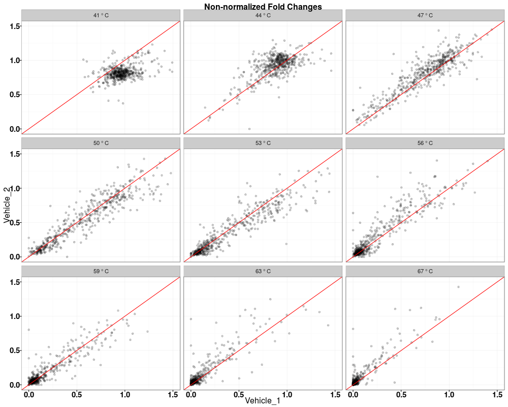
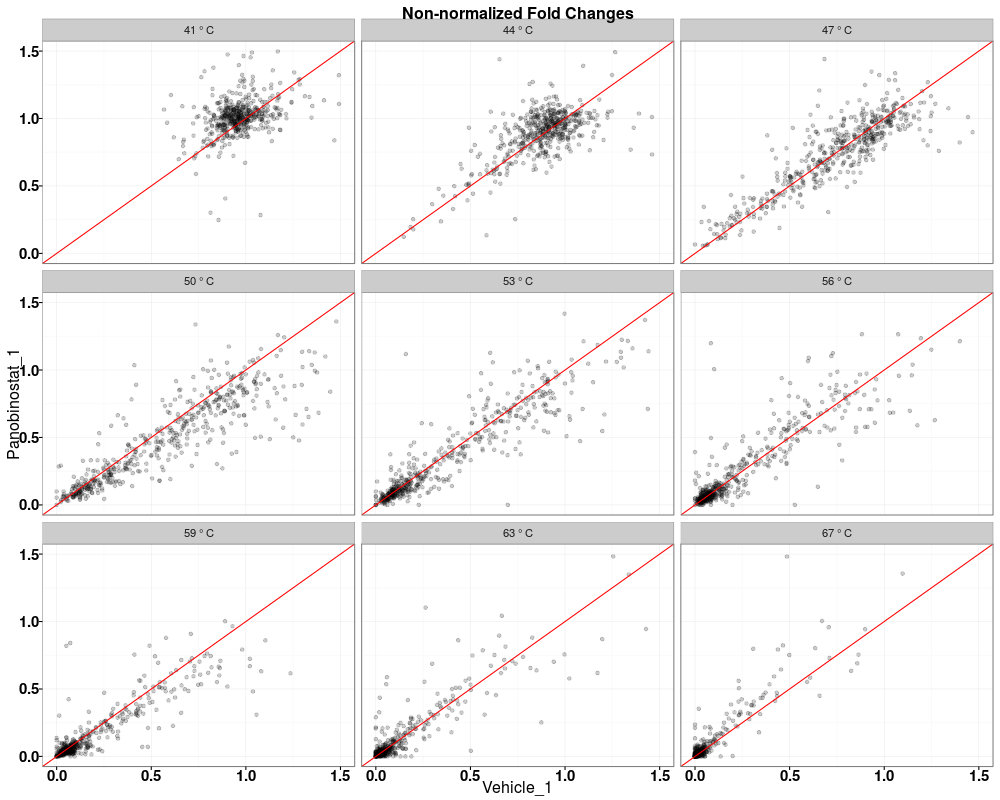
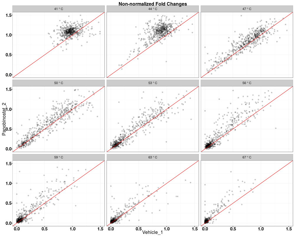
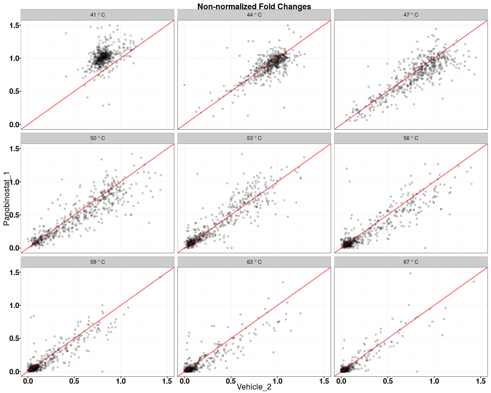
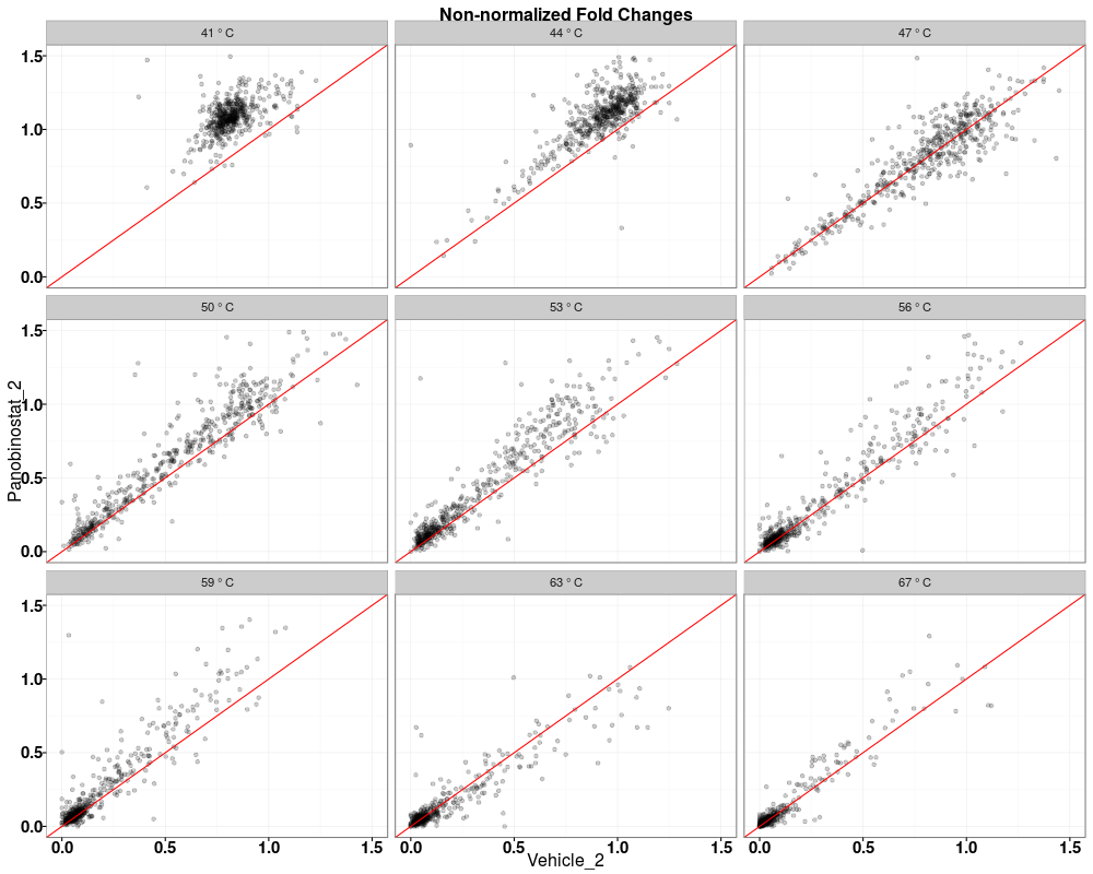
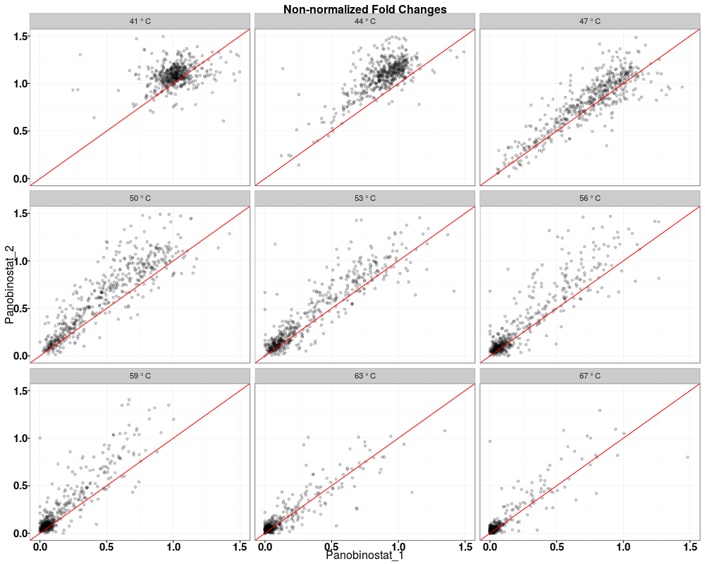
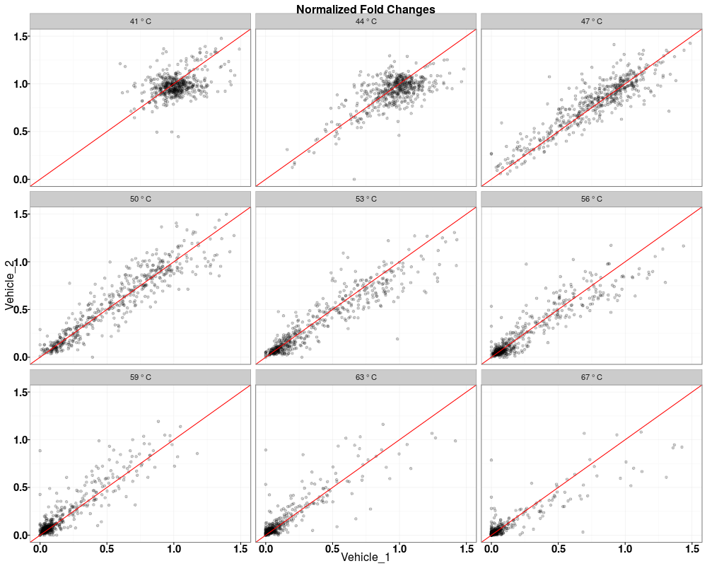
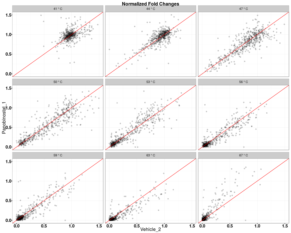
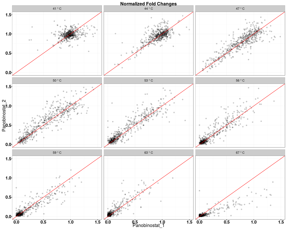
Visually compare fold changes of different TPP experiments.

Description

Plot pairwise relationships between the proteins in different TPP experiments.

Usage

tppQCPlotsCorrelateExperiments(tppData, annotStr = "", path = NULL,
  ggplotTheme = tppDefaultTheme())

Arguments

Value

List of plots for each experiment.

See Also

tppDefaultTheme

Examples

data(hdacTR_smallExample)
tpptrData <- tpptrImport(configTable=hdacTR_config, data=hdacTR_data)
# Quality control (QC) plots BEFORE normalization:
tppQCPlotsCorrelateExperiments(tppData=tpptrData, 
annotStr="Non-normalized Fold Changes")
# Quality control (QC) plots AFTER normalization:
tpptrNorm <- tpptrNormalize(data=tpptrData, normReqs=tpptrDefaultNormReqs())
tpptrDataNormalized <- tpptrNorm$normData
tppQCPlotsCorrelateExperiments(tppData=tpptrDataNormalized, 
annotStr="Normalized Fold Changes")

Results

R version 3.3.1 (2016-06-21) -- "Bug in Your Hair"
Copyright (C) 2016 The R Foundation for Statistical Computing
Platform: x86_64-pc-linux-gnu (64-bit)

R is free software and comes with ABSOLUTELY NO WARRANTY.
You are welcome to redistribute it under certain conditions.
Type 'license()' or 'licence()' for distribution details.

R is a collaborative project with many contributors.
Type 'contributors()' for more information and
'citation()' on how to cite R or R packages in publications.

Type 'demo()' for some demos, 'help()' for on-line help, or
'help.start()' for an HTML browser interface to help.
Type 'q()' to quit R.

> library(TPP)
Loading required package: Biobase
Loading required package: BiocGenerics
Loading required package: parallel

Attaching package: 'BiocGenerics'

The following objects are masked from 'package:parallel':

    clusterApply, clusterApplyLB, clusterCall, clusterEvalQ,
    clusterExport, clusterMap, parApply, parCapply, parLapply,
    parLapplyLB, parRapply, parSapply, parSapplyLB

The following objects are masked from 'package:stats':

    IQR, mad, xtabs

The following objects are masked from 'package:base':

    Filter, Find, Map, Position, Reduce, anyDuplicated, append,
    as.data.frame, cbind, colnames, do.call, duplicated, eval, evalq,
    get, grep, grepl, intersect, is.unsorted, lapply, lengths, mapply,
    match, mget, order, paste, pmax, pmax.int, pmin, pmin.int, rank,
    rbind, rownames, sapply, setdiff, sort, table, tapply, union,
    unique, unsplit

Welcome to Bioconductor

    Vignettes contain introductory material; view with
    'browseVignettes()'. To cite Bioconductor, see
    'citation("Biobase")', and for packages 'citation("pkgname")'.

Loading required package: openxlsx
Loading required package: ggplot2
> png(filename="/home/ddbj/snapshot/RGM3/R_BC/result/TPP/tppQCPlotsCorrelateExperiments.Rd_%03d_medium.png", width=480, height=480)
> ### Name: tppQCPlotsCorrelateExperiments
> ### Title: Visually compare fold changes of different TPP experiments.
> ### Aliases: tppQCPlotsCorrelateExperiments
> 
> ### ** Examples
> 
> data(hdacTR_smallExample)
> tpptrData <- tpptrImport(configTable=hdacTR_config, data=hdacTR_data)
Importing data...

Comparisons will be performed between the following experiments:
Panobinostat_1_vs_Vehicle_1
Panobinostat_2_vs_Vehicle_2


The following label columns were detected:
126, 127L, 127H, 128L, 128H, 129L, 129H, 130L, 130H, 131L.
Importing TR dataset: Vehicle_1
Removing duplicate identifiers using quality column 'qupm'...
508 out of 508 rows kept for further analysis.
  -> Vehicle_1 contains 508 proteins.
  -> 504 out of 508 proteins (99.21%) suitable for curve fit (criterion: > 2 valid fold changes per protein).
Importing TR dataset: Vehicle_2
Removing duplicate identifiers using quality column 'qupm'...
509 out of 509 rows kept for further analysis.
  -> Vehicle_2 contains 509 proteins.
  -> 504 out of 509 proteins (99.02%) suitable for curve fit (criterion: > 2 valid fold changes per protein).
Importing TR dataset: Panobinostat_1
Removing duplicate identifiers using quality column 'qupm'...
508 out of 508 rows kept for further analysis.
  -> Panobinostat_1 contains 508 proteins.
  -> 504 out of 508 proteins (99.21%) suitable for curve fit (criterion: > 2 valid fold changes per protein).
Importing TR dataset: Panobinostat_2
Removing duplicate identifiers using quality column 'qupm'...
509 out of 509 rows kept for further analysis.
  -> Panobinostat_2 contains 509 proteins.
  -> 499 out of 509 proteins (98.04%) suitable for curve fit (criterion: > 2 valid fold changes per protein).


> # Quality control (QC) plots BEFORE normalization:
> tppQCPlotsCorrelateExperiments(tppData=tpptrData, 
+ annotStr="Non-normalized Fold Changes")
$QC_plots_Vehicle_1_vs_Vehicle_2

$QC_plots_Vehicle_1_vs_Panobinostat_1

$QC_plots_Vehicle_1_vs_Panobinostat_2

$QC_plots_Vehicle_2_vs_Panobinostat_1

$QC_plots_Vehicle_2_vs_Panobinostat_2

$QC_plots_Panobinostat_1_vs_Panobinostat_2

> # Quality control (QC) plots AFTER normalization:
> tpptrNorm <- tpptrNormalize(data=tpptrData, normReqs=tpptrDefaultNormReqs())
Creating normalization set:
	1. Filtering by non fold change columns:
Filtering by annotation column(s) 'qssm' in treatment group: Vehicle_1
  Column qssm between 4 and Inf-> 312 out of 508 proteins passed.

312 out of 508 proteins passed in total.

Filtering by annotation column(s) 'qssm' in treatment group: Vehicle_2
  Column qssm between 4 and Inf-> 362 out of 509 proteins passed.

362 out of 509 proteins passed in total.

Filtering by annotation column(s) 'qssm' in treatment group: Panobinostat_1
  Column qssm between 4 and Inf-> 333 out of 508 proteins passed.

333 out of 508 proteins passed in total.

Filtering by annotation column(s) 'qssm' in treatment group: Panobinostat_2
  Column qssm between 4 and Inf-> 364 out of 509 proteins passed.

364 out of 509 proteins passed in total.

	2. Find jointP:
Detecting intersect between treatment groups (jointP).
-> JointP contains 261 proteins.

	3. Filtering fold changes:
Filtering fold changes in treatment group: Vehicle_1
  Column 7 between 0.4 and 0.6 -> 30 out of 261 proteins passed
  Column 9 between 0 and 0.3 -> 223 out of 261 proteins passed
  Column 10 between 0 and 0.2 -> 233 out of 261 proteins passed
22 out of 261 proteins passed in total.

Filtering fold changes in treatment group: Vehicle_2
  Column 7 between 0.4 and 0.6 -> 21 out of 261 proteins passed
  Column 9 between 0 and 0.3 -> 215 out of 261 proteins passed
  Column 10 between 0 and 0.2 -> 227 out of 261 proteins passed
14 out of 261 proteins passed in total.

Filtering fold changes in treatment group: Panobinostat_1
  Column 7 between 0.4 and 0.6 -> 34 out of 261 proteins passed
  Column 9 between 0 and 0.3 -> 217 out of 261 proteins passed
  Column 10 between 0 and 0.2 -> 224 out of 261 proteins passed
21 out of 261 proteins passed in total.

Filtering fold changes in treatment group: Panobinostat_2
  Column 7 between 0.4 and 0.6 -> 15 out of 261 proteins passed
  Column 9 between 0 and 0.3 -> 221 out of 261 proteins passed
  Column 10 between 0 and 0.2 -> 225 out of 261 proteins passed
10 out of 261 proteins passed in total.

Experiment with most remaining proteins after filtering: Vehicle_1
-> NormP contains 22 proteins.
-----------------------------------
Computing normalization coefficients:
1. Computing fold change medians for proteins in normP.
2. Fitting melting curves to medians.
-> Experiment with best model fit: Vehicle_1 (R2: 0.9919)
3. Computing normalization coefficients
Creating QC plots to illustrate median curve fits.
-----------------------------------
Normalizing all proteins in all experiments.
Normalization successfully completed!

> tpptrDataNormalized <- tpptrNorm$normData
> tppQCPlotsCorrelateExperiments(tppData=tpptrDataNormalized, 
+ annotStr="Normalized Fold Changes")
$QC_plots_Vehicle_1_vs_Vehicle_2

$QC_plots_Vehicle_1_vs_Panobinostat_1

$QC_plots_Vehicle_1_vs_Panobinostat_2

$QC_plots_Vehicle_2_vs_Panobinostat_1

$QC_plots_Vehicle_2_vs_Panobinostat_2

$QC_plots_Panobinostat_1_vs_Panobinostat_2

> 
> 
> 
> 
> 
> 
> dev.off()
null device 
          1 
>