R Graphical Manual

Browse All

Last data update: 2014.03.03

R: Transcription Start Site Identification

TSSi-package

R Documentation

Transcription Start Site Identification

Description

The TSSi package normalizes and identifies transcription start sites in high-throughput sequencing data.

Details

High throughput sequencing has become an essential experimental approach for the investigation of transcriptional mechanisms. For some applications like ChIP-seq, there are several available approaches for the prediction of peak locations. However, these methods are not designed for the identification of transcription start sites (TSS) because such data sets have qualitatively different noise.

The TSSi provides a heuristic framework for the identification of TSS based on high-throughput sequencing data. Probabilistic assumptions for the count distribution as well as for systematic errors, i.e. for contaminating measurements close to a TSS, are made and can be adapted by the user. The framework also comprises a regularization procedure which can be applied as a preprocessing step to decrease the noise and thereby reduce the number of false predictions.

The package is published under the GPL-3 license.

Author(s)

Clemens Kreutz, Julian Gehring, Jens Timmer

Maintainer: Julian Gehring <julian.gehring@fdm.uni-freiburg.de>

References

C. Kreutz, J. Gehring, D. Lang, J. Timmer, and S. Rensing: TSSi - An R package for transcription start site identification from high throughput sequencing data.

in preparation

Examples

## load data set
data(physcoCounts)

## segmentize data
attach(physcoCounts)
x <- segmentizeCounts(counts=counts, start=start, chr=chromosome,
region=region, strand=strand)
detach(physcoCounts)

x
segments(x)

## normalize data, w/o and w/ fitting
yRatio <- normalizeCounts(x)
yFit <- normalizeCounts(x, fit=TRUE)
yFit

## identify TSS
z <- identifyStartSites(yFit)
z

## inspect results
head(tss(z, 1))
plot(z, 1)

Results


R version 3.3.1 (2016-06-21) -- "Bug in Your Hair"
Copyright (C) 2016 The R Foundation for Statistical Computing
Platform: x86_64-pc-linux-gnu (64-bit)

R is free software and comes with ABSOLUTELY NO WARRANTY.
You are welcome to redistribute it under certain conditions.
Type 'license()' or 'licence()' for distribution details.

R is a collaborative project with many contributors.
Type 'contributors()' for more information and
'citation()' on how to cite R or R packages in publications.

Type 'demo()' for some demos, 'help()' for on-line help, or
'help.start()' for an HTML browser interface to help.
Type 'q()' to quit R.

> library(TSSi)

Attaching package: 'TSSi'

The following object is masked from 'package:graphics':

    segments

> png(filename="/home/ddbj/snapshot/RGM3/R_BC/result/TSSi/TSSi-package.Rd_%03d_medium.png", width=480, height=480)
> ### Name: TSSi-package
> ### Title: Transcription Start Site Identification
> ### Aliases: TSSi TSSi-package
> ### Keywords: package htest models
> 
> ### ** Examples
> 
> ## load data set
> data(physcoCounts)
> 
> ## segmentize data
> attach(physcoCounts)
> x <- segmentizeCounts(counts=counts, start=start, chr=chromosome,
+ region=region, strand=strand)
> detach(physcoCounts)
> 
> x
* Object of class 'TssData' *
  Data imported

** Segments **
   Segments (5): s1_+_1, s1_+_2, s1_-_3, s2_+_4, s2_-_5
   Chromosomes (2): s1, s2
   Strands (2): +, -
   Regions (5): 1, 2, 3, 4, 5
   nCounts (5): 978, 587, 848, 466, 690

> segments(x)
       chr strand region nPos nCounts   start     end
s1_+_1  s1      +      1   28     978   82747   82994
s1_+_2  s1      +      2   33     587  814741  815042
s1_-_3  s1      -      3   47     848 1435037 1435157
s2_+_4  s2      +      4   68     466 1454505 1455353
s2_-_5  s2      -      5   43     690 1574882 1575467
> 
> ## normalize data, w/o and w/ fitting
> yRatio <- normalizeCounts(x)
> yFit <- normalizeCounts(x, fit=TRUE)
> yFit
* Object of class 'TssNorm' *
  Data normalized

** Segments **
   Segments (5): s1_+_1, s1_+_2, s1_-_3, s2_+_4, s2_-_5
   Chromosomes (2): s1, s2
   Strands (2): +, -
   Regions (5): 1, 2, 3, 4, 5
   nCounts (5): 978, 587, 848, 466, 690

** Parameters **
   pattern: %1$s_%2$s_%3$s
   offset: 10
   basal: 1e-04
   lambda: c(0.1, 0.1)
   fit: TRUE
   optimizer: all

> 
> ## identify TSS
> z <- identifyStartSites(yFit)
> z
* Object of class 'TssResult' *
  TSS in data identified

** Segments **
   Segments (5): s1_+_1, s1_+_2, s1_-_3, s2_+_4, s2_-_5
   Chromosomes (2): s1, s2
   Strands (2): +, -
   Regions (5): 1, 2, 3, 4, 5
   nCounts (5): 978, 587, 848, 466, 690
   nTSS (5): 2, 3, 1, 9, 6

** Parameters **
   pattern: %1$s_%2$s_%3$s
   offset: 10
   basal: 1e-04
   lambda: c(0.1, 0.1)
   fit: TRUE
   optimizer: all
   tau: c(20, 20)
   threshold: 1
   fun: function (fg, bg, indTss, pos, basal, tau, extend = FALSE) 
{
    idx <- pos - pos[1] + 1
    idxTss <- idx[indTss]
    n <- pos[length(pos)] - pos[1] + 1
    fak <- 1/.exppdf(1, tau)
    win1 <- fak[1] * .exppdf(n:1, tau[1])
    win2 <- fak[2] * .exppdf(1:n, tau[2])
    win <- c(win1, 0, win2)
    bgb <- rep(0, n)
    bgb[idxTss] <- bg[indTss]
    cums <- convolve(win, rev(bgb), type = "open")
    expect <- cums[(n + 1):(length(cums) - n)]
    if (!extend) 
        expect <- expect[idx]
    expect[expect < basal] <- basal
    delta <- fg - expect
    delta[delta < 0] <- 0
    res <- list(delta = delta, expect = expect)
    return(res)
}
   readCol: fit
   neighbor: TRUE

> 
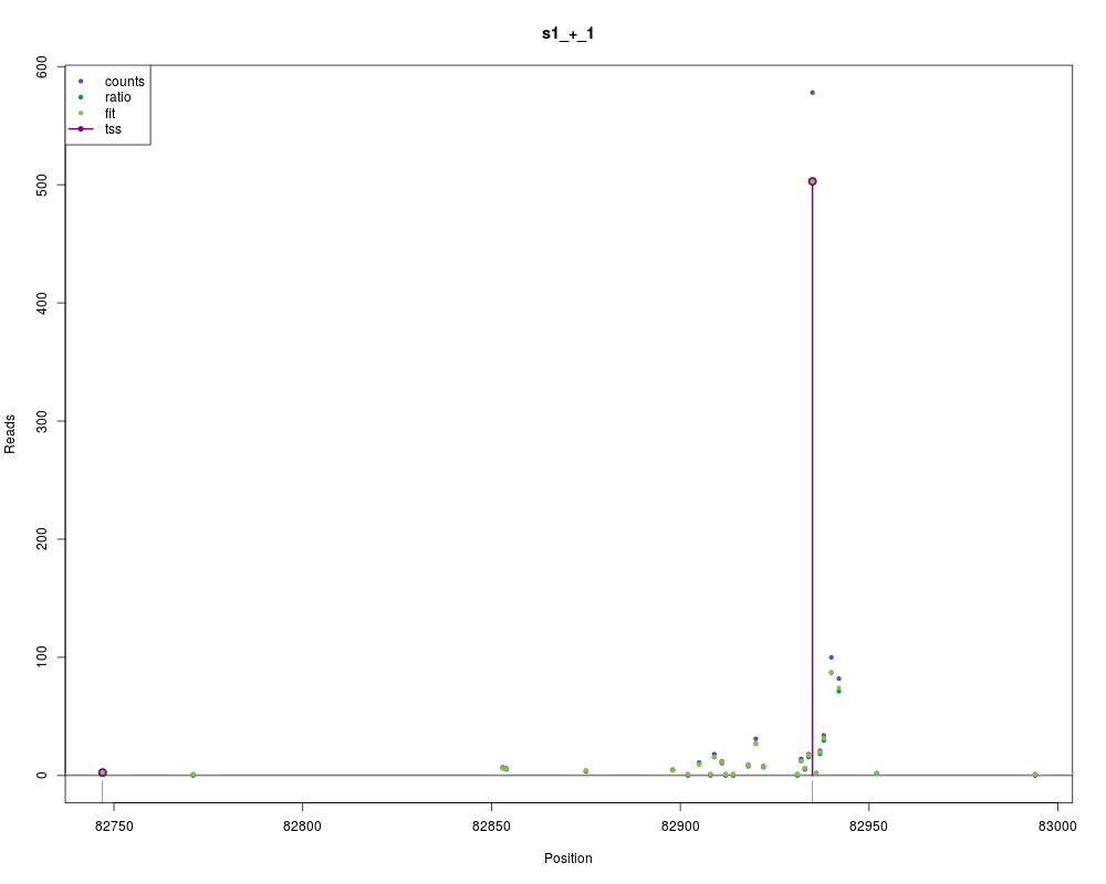
> ## inspect results
> head(tss(z, 1))
    pos      reads
1 82747   2.551251
2 82935 502.836991
> plot(z, 1)
> 
> 
> 
> 
> 
> dev.off()
null device 
          1 
>