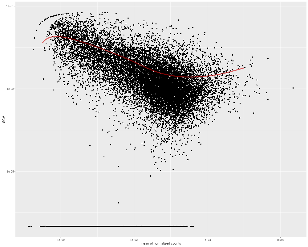
Plot estimated squared coefficient of variation

Description

Plot estimated SCV based on ggplot2

Usage

plotSCVEsts(XB, name = NULL, ymin, linecol = "red3", 
   xlab = "mean of normalized counts", ylab = "SCV")

Arguments

Value

Summary plot for the fitting and estimation of scv

Author(s)

Yuanhang Liu

References

H. I. Chen, Y. Liu, Y. Zou, Z. Lai, D. Sarkar, Y. Huang, et al., "Differential expression analysis of RNA sequencing data by incorporating non-exonic mapped reads," BMC Genomics, vol. 16 Suppl 7, p. S14, Jun 11 2015.

See Also

estimateSCV

Examples

   conditions <- factor(c(rep('C1', 3), rep('C2', 3)))
   data(ExampleData)
   XB <- XBSeqDataSet(Observed, Background, conditions)
   XB <- estimateRealCount(XB)
   XB <- estimateSizeFactors(XB)
   XB <- estimateSCV(XB, fitType='local')
   plotSCVEsts(XB)

Results

R version 3.3.1 (2016-06-21) -- "Bug in Your Hair"
Copyright (C) 2016 The R Foundation for Statistical Computing
Platform: x86_64-pc-linux-gnu (64-bit)

R is free software and comes with ABSOLUTELY NO WARRANTY.
You are welcome to redistribute it under certain conditions.
Type 'license()' or 'licence()' for distribution details.

R is a collaborative project with many contributors.
Type 'contributors()' for more information and
'citation()' on how to cite R or R packages in publications.

Type 'demo()' for some demos, 'help()' for on-line help, or
'help.start()' for an HTML browser interface to help.
Type 'q()' to quit R.

> library(XBSeq)
Loading required package: DESeq2
Loading required package: S4Vectors
Loading required package: stats4
Loading required package: BiocGenerics
Loading required package: parallel

Attaching package: 'BiocGenerics'

The following objects are masked from 'package:parallel':

    clusterApply, clusterApplyLB, clusterCall, clusterEvalQ,
    clusterExport, clusterMap, parApply, parCapply, parLapply,
    parLapplyLB, parRapply, parSapply, parSapplyLB

The following objects are masked from 'package:stats':

    IQR, mad, xtabs

The following objects are masked from 'package:base':

    Filter, Find, Map, Position, Reduce, anyDuplicated, append,
    as.data.frame, cbind, colnames, do.call, duplicated, eval, evalq,
    get, grep, grepl, intersect, is.unsorted, lapply, lengths, mapply,
    match, mget, order, paste, pmax, pmax.int, pmin, pmin.int, rank,
    rbind, rownames, sapply, setdiff, sort, table, tapply, union,
    unique, unsplit


Attaching package: 'S4Vectors'

The following objects are masked from 'package:base':

    colMeans, colSums, expand.grid, rowMeans, rowSums

Loading required package: IRanges
Loading required package: GenomicRanges
Loading required package: GenomeInfoDb
Loading required package: SummarizedExperiment
Loading required package: Biobase
Welcome to Bioconductor

    Vignettes contain introductory material; view with
    'browseVignettes()'. To cite Bioconductor, see
    'citation("Biobase")', and for packages 'citation("pkgname")'.

    Welcome to 'XBSeq'.
> png(filename="/home/ddbj/snapshot/RGM3/R_BC/result/XBSeq/plotSCVEsts.Rd_%03d_medium.png", width=480, height=480)
> ### Name: plotSCVEsts
> ### Title: Plot estimated squared coefficient of variation
> ### Aliases: plotSCVEsts
> 
> ### ** Examples
> 
>    conditions <- factor(c(rep('C1', 3), rep('C2', 3)))
>    data(ExampleData)
>    XB <- XBSeqDataSet(Observed, Background, conditions)
>    XB <- estimateRealCount(XB)
>    XB <- estimateSizeFactors(XB)
>    XB <- estimateSCV(XB, fitType='local')
>    plotSCVEsts(XB)
> 
> 
> 
> 
> 
> dev.off()
null device 
          1 
>