Supported by Dr. Osamu Ogasawara and  . . |
|
Last data update: 2014.03.03 |
Fitting a smooth curve through paired (x,y) dataDescriptionFitting a smooth curve through paired (x,y) data. Usage
## S3 method for class 'matrix'
fitXYCurve(X, weights=NULL, typeOfWeights=c("datapoint"), method=c("loess", "lowess",
  "spline", "robustSpline"), bandwidth=NULL, satSignal=2^16 - 1, ...)
Arguments
ValueA named Missing valuesThe estimation of the function will only be made based on complete
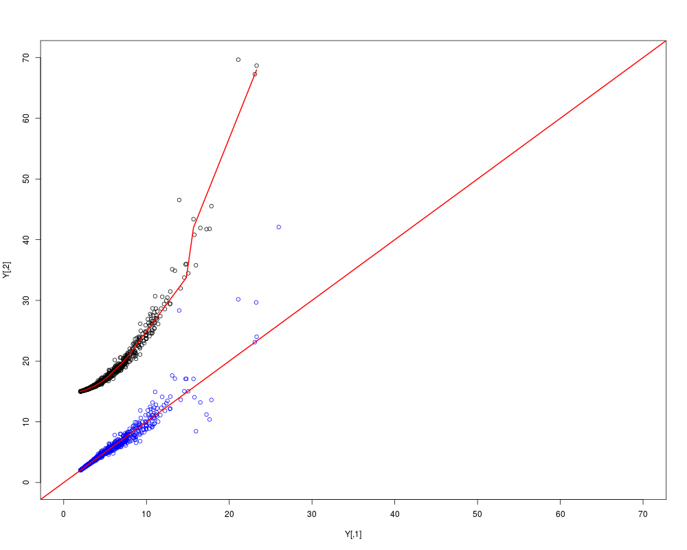
non-saturated observations, i.e. observations that contains no Weighted normalizationEach data point, that is, each row in Note that the lowess and the spline method only support zero-one {0,1} weights. For such methods, all weights that are less than a half are set to zero. Details on loessFor Author(s)Henrik Bengtsson Examples# Simulate data from the model y <- a + bx + x^c + eps(bx) x <- rexp(1000) a <- c(2,15) b <- c(2,1) c <- c(1,2) bx <- outer(b,x) xc <- t(sapply(c, FUN=function(c) x^c)) eps <- apply(bx, MARGIN=2, FUN=function(x) rnorm(length(x), mean=0, sd=0.1*x)) Y <- a + bx + xc + eps Y <- t(Y) lim <- c(0,70) plot(Y, xlim=lim, ylim=lim) # Fit principal curve through a subset of (y_1, y_2) subset <- sample(nrow(Y), size=0.3*nrow(Y)) fit <- fitXYCurve(Y[subset,], bandwidth=0.2) lines(fit, col="red", lwd=2) # Backtransform (y_1, y_2) keeping y_1 unchanged YN <- backtransformXYCurve(Y, fit=fit) points(YN, col="blue") abline(a=0, b=1, col="red", lwd=2) Results
R version 3.3.1 (2016-06-21) -- "Bug in Your Hair"
Copyright (C) 2016 The R Foundation for Statistical Computing
Platform: x86_64-pc-linux-gnu (64-bit)

R is free software and comes with ABSOLUTELY NO WARRANTY.
You are welcome to redistribute it under certain conditions.
Type 'license()' or 'licence()' for distribution details.

R is a collaborative project with many contributors.
Type 'contributors()' for more information and
'citation()' on how to cite R or R packages in publications.

Type 'demo()' for some demos, 'help()' for on-line help, or
'help.start()' for an HTML browser interface to help.
Type 'q()' to quit R.

> library(aroma.light)
aroma.light v3.2.0 (2016-01-06) successfully loaded. See ?aroma.light for help.
> png(filename="/home/ddbj/snapshot/RGM3/R_BC/result/aroma.light/fitXYCurve.Rd_%03d_medium.png", width=480, height=480)
> ### Name: fitXYCurve
> ### Title: Fitting a smooth curve through paired (x,y) data
> ### Aliases: fitXYCurve fitXYCurve.matrix backtransformXYCurve
> ###   backtransformXYCurve.matrix
> ### Keywords: methods
>
> ### ** Examples
>
>  # Simulate data from the model y <- a + bx + x^c + eps(bx)
> x <- rexp(1000)
> a <- c(2,15)
> b <- c(2,1)
> c <- c(1,2)
> bx <- outer(b,x)
> xc <- t(sapply(c, FUN=function(c) x^c))
> eps <- apply(bx, MARGIN=2, FUN=function(x) rnorm(length(x), mean=0, sd=0.1*x))
> Y <- a + bx + xc + eps
> Y <- t(Y)
>
> lim <- c(0,70)
> plot(Y, xlim=lim, ylim=lim)
>
> # Fit principal curve through a subset of (y_1, y_2)
> subset <- sample(nrow(Y), size=0.3*nrow(Y))
> fit <- fitXYCurve(Y[subset,], bandwidth=0.2)
>
> lines(fit, col="red", lwd=2)
>
> # Backtransform (y_1, y_2) keeping y_1 unchanged
> YN <- backtransformXYCurve(Y, fit=fit)
> points(YN, col="blue")
> abline(a=0, b=1, col="red", lwd=2)
>
>
>
>
>
>
> dev.off()
null device
          1
>
|